Visualizing algorithm growth rates

I have been singing paeans about ‘R’, the statistics language, in this blog because it helps one understand and code statistical programs which are the key to various calculations in the fields of project management and capacity planning.
I have also been mulling about how I can generate graphs of algorithm growth rates when input sizes vary. This is child’s play when we use ‘R’.

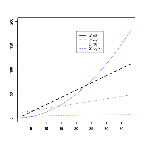
I could reproduce the graph from Jones and Bartlett’s ‘Analysis of Algorithms’ quite easily. Visualizing these growth rates easily like this is helpful.

The code is general. Nothing specific to algorithm analysis. Immensely useful.

png("funcgrowth.png")
curve(x*x/8,xlab="",ylab="",col="blue",ylim=c(0,200),xlim=c(2,38))
par(new=TRUE)
curve(3*x-2,lwd=3,ylim=c(0,200),xlab="",ylab="",xlim=c(2,38),lty="dashed")
par(new=TRUE)
curve(x+10,lty="dashed",lwd=1,ylim=c(0,200),xlab="",ylab="",xlim=c(2,38))
par(new=TRUE)
curve(2*log(x),col="blue",lty="dashed",lwd=1,ylim=c(0,200),xlab="",ylab="",xlim=c(2,38))
legend(20,180, c("x*x/8","3*x-2","x+10","2*log(x)"), lty=c(1,2,2,2), lwd=c(2.5,2.5,1,1),col=c("blue","black","black","blue"))
dev.off()

‘atoi’ function code kata

I recently coded the ‘atoi’ function in Java as part of an assignment while I was reading ‘Hacker’s delight’, a delightful book full of bit twiddling tricks and techniques.
These ideas reduce the number of instructions used to execute code and should be followed by Java coders who work on critical transaction processing applications to increase throughput.

package com.atoi;

import java.math.BigInteger;

import static junit.framework.Assert.assertEquals;

/**
 * User: Mohan Radhakrishnan
 * Date: 10/21/12
 * Time: 1:19 PM
 */
public class Atoi {

    /**
     * Convert 'char' to 'int'.
     * @param chars
     * @return result final result or result till an ASCII space
     *         if encountered.
     */
    public int atoi( char[] chars ) {

        assert( chars != null && chars.length != 0 );
        int i = 0;
        int result = 0;
        char temp = 0;

        while( i < chars.length ){
            if( (chars[ i ] ^ 0x20)  == 0 ){
                return result;//Stop at the first ASCII space
            }else if ( isBetween0And9( chars[ i ] - '0')){
                //calculate
                result = ( result * 10 ) + ( chars[ i ] - '0');
            }
            i++;
        }
        return result;

    }

    /**
     * Referred 'Hacker's delight' which
     * has bit techniques that helps in reducing
     * instructions.
     * If the result of this bit twiddling is 0x80808080
     * then the input is less than 9
     * The advantage is that a extensible function to find
     * any range can be coded with slight modification.
     * @param input
     * @return result of the check
     */

    public boolean isBetween0And9(int input){
        System.out.println(  "isBetween0And9 [" + Integer.toBinaryString( input ) + "]");
        int y = ( input & 0x7F7F7F7F ) + 0x76767676;
        y = y | input;
        y = y | 0x7F7F7F7F;
        y = ~y;
        System.out.println( "~y [" + Integer.toBinaryString( y ) + "]");
        return( 0x80808080 == y );

    }
}

I also coded JUnit tests mainly to test the logic from “Hacker’s Delight’ that checks for a overflow before it occurs. That was interesting because I could check if an ‘int’ exceeds Integer.MAX_INT or underflows without using the Java libraries or checked exceptions. Since this code is not simple to understand I coded it and tested it but didn’t copy it into this entry. Later.

public class AtoiTest {
    
    @Test
    public void testAtoi() throws Exception {
        Atoi atoi = new Atoi();
        try{
            assertEquals( 5, atoi.atoi( new char[] {'5'}));
            assertEquals( 0, atoi.atoi( new char[] {'A'}));
            assertEquals( 5, atoi.atoi( new char[] {'5','A'}));
            assertEquals( 5, atoi.atoi( new char[] {'A','5'}));
            assertEquals( 0, atoi.atoi( new char[] {' ','5'}));
            assertEquals( 56, atoi.atoi( new char[] {'5','6',' ','5'}));
            assertEquals( 506, atoi.atoi( new char[] {'5','0','6',' ','5'}));
        }catch ( Exception e){
            fail();
        }
    }
}

Github code

I started to push code into Github. Skiplists were invented by William Pugh and I looked at the ‘C’ code available at ftp.cs.umd.edu and coded Java programs. I am trying to code algorithms and a Skiplist was the first one. This code might not be the best but it will be refactored.
If I am able to sustain this motivation I will code graph algorithms and other data structures. Initially I was interested in distributed algorithms but they require special skills to understand.

Statistics of agreement

I found this formula that calculates the percentage of agreement between two ratings quite interesting and coded the following simple steps using ‘R’. This is called Cohen’s kappa and even though there is nothing original about this entry it is very useful. I wrote the simple R code though because I am learning R.
It was also surprising that I didn’t know about it and our teams are not at all technical enough even to use these foundational principles. As is evident this has wide applications in the fields of percentage agreement calculations when two teams don’t agree or auditors don’t agree with each other. Whither will our antagonistic attitude towards good calculations in technical and project management drive us.

The other point that is a highlight is that I found the description of this formula in a paper dealing with Architecture Trade-off Analysis Method.

The matrix created below shows that two people agree with each other on certain points and disagree on others. The formula to calculate the level of agreement is

Observed percentage of agreement - Expected percentage of agreement
--------------------------------------------------------------
1 - Expected percentage of agreement

R code

kappa<-matrix(c(5,2,1,2),ncol=2)
colnames(kappa)<-c("Disagree","Agree")
rownames(kappa)<-c("Disagree","Agree")
kappa

( I have formatted the output of 'R' as a table )


DisagreeAgree
Disagree51
Agree22

kappamargin<-kappa/margin.table(kappa)
kappamargin

( I have formatted the output of 'R' which are the percentages as a table )


DisagreeAgree
Disagree0.50.1
Agree0.20.2

Observed percentage of agreement = 0.5 + 0.2

Now we want the totals as this table shows. We multiply the total figures of the same color


AgreeDisagreeTotal
Agree0.50.10.6
Disagree0.20.20.4
Total0.70.3

So I have just used this line of code to create a matrix of the totals for illustration.

marginals<-matrix(c(margin.table(kappamargin,1),margin.table(kappamargin,2)),ncol=2)
marginals

( I have formatted the output of 'R' as a table )


0.60.7
0.40.3

Expected percentage of agreement = ( 0.6 * 0.7 ) + ( 0.4 * 0.3 )

So final kappa value is

(0.7 - (marginals[1,1] * marginals[1,2]) + (marginals[2,1] * marginals[2,2])) /
(1- (marginals[1,1] * marginals[1,2]) + (marginals[2,1] * marginals[2,2]))

0.57

(i.e)

0.7 - (( 0.6 * 0.7 ) + ( 0.4 * 0.3 ))
----------------------------------
1 - (( 0.6 * 0.7 ) + ( 0.4 * 0.3 ))

Throughput and Response time curves using R

I started using ‘R’, the statistical language, recently but its power is sorely missed in the IT industry especially in the project management and Capacity planning fields. In fact rigorous data quantification and analysis is given the short shrift by us in our software management activities like calculation of schedule variance and trends.

‘R’ in combination with PDQ helps us visualize the throughput and response time data. We should also be able to predict future performance by changing the service demands assuming that a faster disk or CPU is added. But that is a slightly more involved exercise.

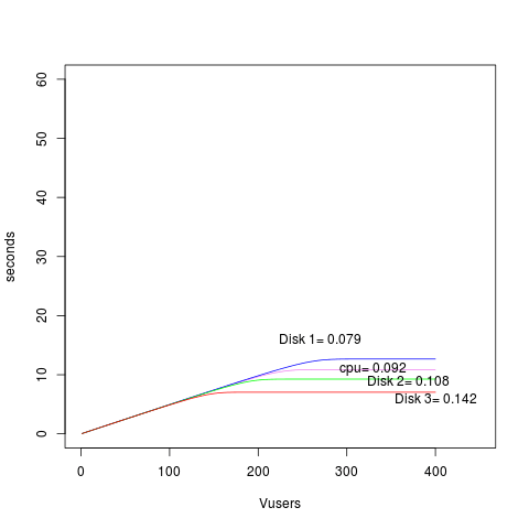
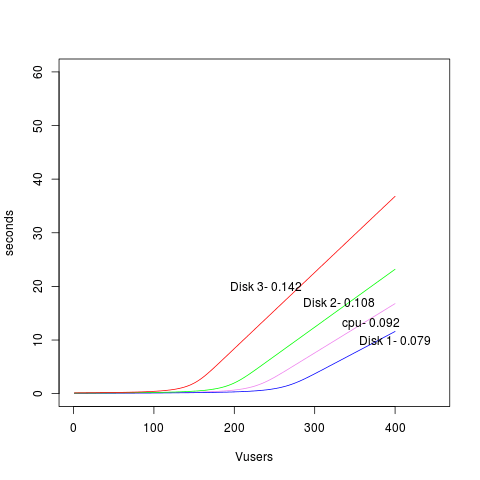
This simple script shows response time graphs of multiple devices in the same graph.

The second graph shows throughput curves. We just have to use GetThruput instead of GetResponse.

library(pdq)

# PDQ globals
load<-400
think<-20

cpu<-"cpunode"
disk1<-"disknode1"
disk2<-"disknode2"
disk3<-"disknode3"


cpudemand<-0.092
disk1demand<-0.079
disk2demand<-0.108
disk3demand<-0.142

workload<-"workload"

# R plot vectors
xc<-0
yc<-0

for (n in 1:load) {
	Init("")

	CreateClosed(workload, TERM, as.double(n), think)

	CreateNode(cpu, CEN, FCFS)
	SetDemand(cpu, workload, cpudemand)

	Solve(EXACT)

	xc[n]<-as.double(n)
	yc[n]<-GetResponse(TERM, workload)
}
plot(xc, yc, type="l", ylim=c(0,60), xlim=c(0,450), lwd=1, xlab="Vusers", ylab="seconds",col="violet")

text(370,13,paste("cpu-",as.numeric(cpudemand)))

# R plot vectors
xc1<-0
yc1<-0

for (n in 1:load) {
	Init("")

	CreateClosed(workload, TERM, as.double(n), think)

	CreateNode(disk1, CEN, FCFS)
	SetDemand(disk1, workload, disk1demand)

	Solve(EXACT)

	xc1[n]<-as.double(n)
	yc1[n]<-GetResponse(TERM, workload)
}
lines(xc1, yc1,lwd=1,col="blue")
text(400,10,paste("Disk 1-",as.numeric(disk1demand)))

# R plot vectors
xc2<-0
yc2<-0

for (n in 1:load) {
	Init("")

	CreateClosed(workload, TERM, as.double(n), think)

	CreateNode(disk2, CEN, FCFS)
	SetDemand(disk2, workload, disk2demand)

	Solve(EXACT)

	xc2[n]<-as.double(n)
	yc2[n]<-GetResponse(TERM, workload)
}
lines(xc2, yc2,lwd=1,col="green")
text(330,17,paste("Disk 2-",as.numeric(disk2demand)))

# R plot vectors
xc3<-0
yc3<-0

for (n in 1:load) {
	Init("")

	CreateClosed(workload, TERM, as.double(n), think)

	CreateNode(disk3, CEN, FCFS)
	SetDemand(disk3, workload, disk3demand)

	Solve(EXACT)

	xc3[n]<-as.double(n)
	yc3[n]<-GetResponse(TERM, workload)
}
lines(xc3, yc3,lwd=1,col="red")
text(240,20,paste("Disk 3-",as.numeric(disk3demand)))

Load vs Response

Load vs Throughput

Performance engineering – Simple Bottleneck analysis

I believe the software developers and leads have forgotten the fundamental concepts of Statistics and other indispensable foundational derivations and formulae. One of the key reasons for this is succinctly explained by Cary V. Millsap from Oracle Corporation in his paper “Performance Management : Myths and Facts”.

“The biggest obstacle to accurate capacity planning is actually the difficulty in obtaining usable workload forecasts. Ironically, the difficulty here doesn’t stem from a lack of mathematical sophistication at all, but rather from the inability or unwillingness of a business to commit to a program of performance management that includes testing, workload management, and the collection and analysis of data describing how a system is being used. “

I am learning the ropes here but one field that is very helpful for performance engineering is queuing theory and analysis and the following is a collection of details from various papers. There is also a rather feeble attempt by me to use PDQ for solving a simple queuing problem.

Fundamentals :

T–the length of the observation period;
A–the number of arrivals occurring during
the observation period;
B–the total amount of time during which the system is busy during the observation period (B ≤ T); and
C–the number of completions occurring during the observation period.

Four important derived quantities are
λ = A/T, the arrival rate (jobs/second);
X = C/T, the output rate (jobs/second);
U = B/T, the utilization (fraction of time system is busy); and
S = B/C, the mean service time per completed job.

My feeble attempt to solve a particular problem. The resulting graph seems erroneous at this time but I will try to fix it.

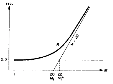
Problem statement from pages 241-242 in “The Operational Analysis of Queueing Network Models* by PETER J. DENNING and JEFFREY P. BUZEN (Computing Surveys, Vol. 10, No. 3, September 1978)

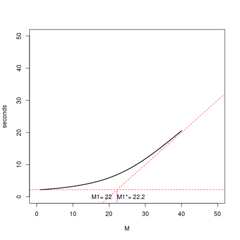
using pdq and get the graph

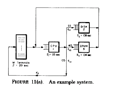
based on the system diagram

The diagram is smudged. The think time, Z is 20 seconds and S1 = 05 seconds, S2 = 08 seconds and S3 = 04 seconds.

The visit ratios( mean number of requests per job for a device ) shown in the diagram and given in the paper are

V0 = 1 = .05V1
Vl = V0 + V2 + V3
v2 = .55V1
V3 = .40V1

Solving these equations we get these values. The paper shows the result but it is trivial to substitute and derive the results. So I have done that.

v1 = .05(v2/.55) + .55(v2/.55) + .40(v2/.55)

v1 = v2/.55

v1 = ( v2 * 100 ) /55

55v1 = 100v2

11v1 = 20 v2

v1/ v2 = 20/11

v3 = v1 – v0 – v2

v3 = .40 * 20 v2 / 11

11v3 = 8v2

v2/v3 = 8/11

V1 * S1 = (20)(.05) = 1.00 seconds (Total CPU time is the bottleneck )

V2 * S2 = (11)(.08) = .88 seconds (Total Disk time)

V3 * S3 = (8)(.04)= .32 seconds (Total Drum time)

These products sum to the minimal response time of 2.2 seconds

V1 * S1 = (20)(.05) = 1.00 seconds (Total CPU time is the bottleneck )

V2 * S2 = (11)(.08) = .88 seconds (Total Disk time)

V3 * S3 = (8)(.04)= .32 seconds (Total Drum time)

These products sum to the minimal response time of 2.2 seconds

The number of terminals required to begin saturating the entire system is
Ml* = 22.2

My feeble attempt to use PDQ based on many resources.

# Bottleneck analysis .

library(pdq)

# PDQ globals
load<-40
think<-20

cpu<-"cpunode"
disk<-"disknode"
drum<-"drumnode"

cpustime<-1.00
diskstime<-.88
drumstime<-.32
dstime<-15

workload<-"workload"

# R plot vectors
xc<-0
yc<-0

for (n in 1:load) {
	Init("")

	CreateClosed(workload, TERM, as.double(n), think)

	CreateNode(cpu, CEN, FCFS)
        #SetVisits(cpu, workload, 20.0, cpustime)
	SetDemand(cpu, workload, cpustime)


	CreateNode(disk, CEN, FCFS)
	SetDemand(disk, workload, diskstime)

	CreateNode(drum, CEN, FCFS)
	SetDemand(drum, workload, drumstime)


	Solve(EXACT)

	xc[n]<-as.double(n)
	yc[n]<-GetResponse(TERM, workload)
}

M1<-GetLoadOpt(TERM, workload)

plot(xc, yc, type="l", ylim=c(0,50), xlim=c(0,50), lwd=2, xlab="M", ylab="seconds")
abline(a=-think, b=cpustime, lty="dashed",  col="red") 
abline( 2.2, 0, lty="dashed",  col = "red")
text(18, par("usr")[3]+2, paste("M1=", as.numeric(M1)))

# This calculation is from the x and y values used to draw lines above
# y = -think + x
# 2.2 = -20 + x
x = 22.2
segments( x, par("usr")[3], x, 2.2, col="violet", lwd=2)
text(26, par("usr")[3]+2, paste("M1*=", x))

Points

1. I was trying to set the visits( mean number of requests per job for a device ) to get an exact graph. Initially I did not know how to do that. Point 2 below seems to be what I missed initially.

2. The graph I got seemed to be wrong because the value of M1 and M1* described in the paper and shown above are wrongly calculated. M1* is the straight line drawn from the intersection of the two dashed red lines to intersect the Y-axis.

2. The new graph is a result of the new service demands

cpustime<-1.00
diskstime<-.88
drumstime<-.32

each of which is set to the product of the visit time and service time. M1 and M1* seem to be close to the problem graph in the paper.

3. The additional point is that I might have made an error in the PDQ or R code that I have failed to detect. I am not still an expert. The asymptote intersects the y-axis before ’20’ but the value of M1 is 22. That looks like an error which I will try to figure out.

Software Architecture evaluation

I wrote to the authors of “Scaling Architecture Evaluations Within Real-World Constraints” about my interest in finding reference material for the various Software Architecture evaluation methods like ATAM, CBAM etc.

One of the authors, Zhao li, responded with a rather large list of references. I have not read all of them. Now that I have found references I am searching for companies that actualy use one or many of them !!

Scenario-based Architecture Evaluation

ALMA Architecture Level Modifiability Analysis  [32]
ALPSM Architecture Level Prediction of Software Maintenance [33]
ATAM Architecture Trade-Off Analysis Method [13]
ARID Active Review for Intermediate Design [21]
CBAM Cost Benefit Analysis Method [22]
CPASA Continuous Performance Assessment of Software Architecture [23]
ESAAMI Extending SAAM by Integration in the Domain [19]
HoPLAA TAM for Production Line Analysis [20]
SAAM Scenario-based Architecture Analysis Method [15]
SAAMCS SAAM Founded on Complex Scenarios [18]
SAAMER Software Architecture Analysis Method for Evolution and Reusability [34]
SALUTA Scenario-based Architecture Level Usability Analysis [35]
AHP Analytic hierarchy process [28]

Attribute-based Software Architecture Evaluation

ALRRA Architecture Level Reliability Risk Analysis [29]
PASA Performance Assessment of Software Architectures [10]
SAEM Software Architecture Evaluation Model [9]
SAABNet Software Architecture Evaluation Model [11]
SACMM Metrics of Software Architecture Changes based on Structural Metrics [27]
SASAM Static Evaluation of Software Architecture [25]

Others

ISAR Independent Software Architecture Review [24]
GQM Application of Goal/Question/Metric framework on SA [26]
LAAAM Lightweight Architecture Alternative Analysis Method [30]
TARA Tiny Architecture Review Approach [31]

REFERENCES

1.        L. Bass, P. Clements, and R. Kazman, “Software Architecture in Practice.” Addison-Wesley, 1998

2.        W. Li and S. Henry, “Object-Oriented Metrics that Predict Maintainability,” J. Systems and Software, vol. 23, no. 2. pp. 111-122, Nov. 1993.

3.        L. Dobrica and E. Niemela, “A Survey on Software Architecture Analysis Methods”, IEEE Transactions on Software Engineering, Vol. 28, No. 7, July 2002

4.        Y. Chen, X. Li, L. Yi, “A Ten-Year Survey of Software Architecture,” IEEE International Conference on Software Engineering and Service Science (ICSESS), 2010

5.        Microsoft, “Analyzing Requirements and Defining Microsoft .Net Solution Architectures,” MCSD Self-Paced Training Kit, Microsoft 2003.

6.        Z. Li, “Internal individual Interviews with Architect in ABB CRC,” June, 2011.

7.        M. Lopez, “Application of an evaluation framework for analyzing the architecture tradeoff analysis method,” The J. of System and Software Vol. 68, No. 3, Dec 2003.

8.        K. Skadron, M. Martonosi, D. August “Challenges in Computer Architecture Evaluation,” Computer, 2003.

9.        J. C. Duenas, W. L. de Oliveira, and J. A. de la Puente, “A Software Architecture Evaluation Model,” Proc. Second Int’l ESPRIT ARES Workshop, pp. 148-157, Feb. 1998.

10.        L. G. Williams, C. U. Smith, “Performance Evaluation of Software Architectures.” Proc. of the 1st Int’l Workshop on Software and Performance.New York: ACM Press, 2002. 179-189

11.        Van Gurp J., J. Bosch , “Automating software architecture assessment”, Proc. of the 9th Nordic Worship on Programming and Software Development Environment Research. Lillchammer, 2000.

12.        J. Bosch and P. Molin, “Software Architecture Design: Evaluation and Transformation,” Proc. IEEE Eng. Of Computer Based Systems Symp., Dec. 1999

13.        P. Clements, R. Kazman, M. Klein, “Evaluating Software Architectures, methods and case studies”, Addison-Wesley, 2002

14.        R. Kazman,  G. Abowd, L.Bass, and M.Webb, “Analyzing the Properties of User Interface Software Architectures,” Technical Report, CMU-CS-93-201, Carnegie Mellon Univ.,SchoolofComputerScience, 1993.

15.        R. Kazman, G. Abowd, L. Bass, and P. Clements, “Scenario-Based Analysis of Software Architecture,” IEEE Software, Nov. 1996.

16.        R. Kazman,  G. Abowd, L.Bass, and M.Webb, “Analyzing the Properties of User Interface Software Architectures,” Technical Report, CMU-CS-93-201, Carnegie Mellon Univ.,SchoolofComputerScience, 1993.

17.        R. Kazman, M. Klein, M. Barbacci, H. Lipson, T. Longstaff, and S.J. Carriere, “The Architecture Tradeoff Analysis method,” Proc. Fourth Int’l Conf. Eng. Of Complex Computer Systems (ICECCS’ 98), Aug. 1998.

18.        N. Lassing, D. Rijsenbrij, and H. van Vliet, “On Software Architecture Analysis of Flexibility, Complexity of Changes: Size Isn’t Everything,” Proc. Second Nordic Software Architecture Workshop, 1999

19.        G. Molter, “Integrating SAAM in Domain-Centric and Reuse-Based Development Processes,” Proc. Second Nordic Workshop Software Architecture (NOSA’ 99)

20.        F. G. Olumofin and V. B. Misic, “Extending the ATAM Architecture Evaluation to Product Line Architectures”, Technical report TR 05/02 Department of computer science, university of Manitoba Winnipeg, Manitoba, Canada R3T 2N2, June 2005

21.        P. Clements, SEI, CMU, http://www.sei.cmu.edu/architecture/tools/arid/ 2000

22.        R. Kazman, J. Asundi, M. H. Klein, SEI, CMU, http://www.sei.cmu.edu/architecture/tools/cbam/ 2002

23.        R.J. Pooley, and A.A.L. Abdullatif, “CPASA: Continuous Performance Assessment of Software Architectur,” Engineering of Computer-based Systems, IEEE International Conference on the Engineering of Computer-Based Systems, 2010.

24.        A. Tang, F.-C Kuo and M.F. Lau “Towards Independent Software Architecture Review,” in 2nd European Conference on Software Architecture, 2008

25.        J. Knodel, M. Lindvall, D. Muthig, M. Naab  “Static evaluation of software architecture.” Proc. of the conf. on Software Maintenance and Reengineering (CSMR 2006).

26.        A. Zalewski, “Beyond ATAM: Architecture Analysis in the Development of Large Scale Software Systems,” Lecture Notes in Computer Science, 2007.

27.        T. Nakamura, V. R. Basili “Metrics of software architecture changes based on structural distance.” In Proc. of the 11th IEEE Int’l Software Metrics Symp.

28.         L. M. Zhu, A. Aurum, “Tradeoff and sensitivity analysis in software architecture evaluation using analytic hierarchy process,” Software Quality Journal, 2005.

29.        S. M.Yacoub and H. H. Ammar “A methodology for architecture-level reliability risk analysis.” IEEE Trans. On Software Engineering, 2002

30.        S.J. Carriere, Lightweight Architecture Alternative Assessment Method, http://technogility.sjcarriere.com/2009/05/11/its-pronounced-like-lamb-not-like-lame.

31.        E. Woods “Industrial Architectural Assessment using TARA.”, 2011 Ninth Working IEEE/IFIP Conference on Software Architecture, 2011

32.        P. Bengtsson, P. N. Lassing, J. Bosch, and H. van Vliet “Architecture-Level Modifiability Analysis (ALMA)” Journal of System and Software, 2004.

33.        P. Bengtsson and J. Bosch, “Architecture Level Prediction of Software Maintenance,” Proc. Third European conf. Software Maintenance and Reeng., 1999

34.        C. Lung, S.Bot, K.Kalaichelvan, and R.Kazman, “An Approach to Software Architecture Analysis for Evolution and Reusability,” Proc. CASCON’97, Nov. 1997.

35.        E. Folmer, J. van Gurp, and J. Bosch, “Software Architecture Analysis of Usability.” Proc EHCI-DSVIS2004, Springer LNCS Vol. 3425, 2005

36.        IEEE 1061, “IEEE standard for a Software Quality Metrics”, IEEE, 1998

37.        Karen Smiley and Jiang Zheng, “Writing strong functional and nonfunctional requirements”, ABB Internal training 2011
Wicked problems

The project management that is widely prevalent in IT firms in my region is simple but extremely, uncontrollably and irretrievably messy. Why is it simple ? It is simple because it is equated with people management which is a social factor. So the technical complexities like WBS, resource loading and leveling, establishment of soft and hard constraints, float analysis, Confidence Intervals etc. are coolly swept under the carpet and the whole structure is transformed into an endless series of meetings, mails and intractable egoistic problems that defy solutions.

Project management is a ‘Wicked problem’  – such as it is. Now its transmutation into people issues makes it a bewildering array of wickedness. So now even projects executed on a smaller scale are not tame problems at all .

We need to read and understand its morphology. The criteria mentioned by this Swedish Morphological Society applies to this type of project management.

Weaving java.util.concurrent API using AspectJ

I stopped using AspectJ long back because we were not really coding aspects because it required an enormous amount of effort to train others. But recently I wrote this to weave into java.util.concurrent libraries to try to explore how the ForkJoin library works. Even though the code works I thought it is not a recommended way to weave into libraries dealing with concurrency written by experts. I pulled  the source and created a custom JAR and used -Xbootclasspath to make it work.


@Aspect
public class ForkJoinProjector {


    @Pointcut( "execution ( int java.util.concurrent.ForkJoinPool.registerWorker(java.util.concurrent.ForkJoinWorkerThread)) &&" +
			                " args(thread) &&" +
			                " target(pool)" )
    public void buildQueues( ForkJoinWorkerThread thread,
	                     ForkJoinPool pool){}
	
    @After("buildQueues( thread,pool)")
    public void build( ForkJoinWorkerThread thread,
    		           ForkJoinPool pool ) {
    	System.out.println( "ID " + thread.getId() + " Name " + thread.getName() );
    }


}

The Alan Turing Year

Image

I am watching the UEFA match between Poland and Greece and ruing the lack of professional ethics in the project management community and the great divide that exists between them and the technical team and I came across The Alan Turing Year. There is a flood of information here.