R Reference classes

A pure OO approach and a functional representation of it are at loggerheads. That is evident when one tries to adopt an OO approach using a powerful functional language. That is my personal opinion.

R has many Object-oriented features built into it.

R has three object oriented (OO) systems: [[S3]], [[S4]] and [[R5]].

Reference classes are one such feature.

OO

Let us consider this data. The id is that of a Subject who is in
a room where monitoring equipment gathers some data. There are several visits to gather this data.

id visit room value timepoint
14 0 bedroom 6 53
14 0 bedroom 6 54
15 0 bedroom 2.75 56

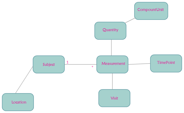
The idea that this code is based on is from Martin Fowler’s book Analysis Patterns Reusable Object Models. The chapter on Observations and Measurements has a diagram roughly equivalent to the
one shown at the top.

The code is lightly tested several times but without unit tests.

library(plyr)
library(dplyr)
library(purrr)

CompoundUnit <- setRefClass("CompoundUnit",
fields = list(micrograms = 'numeric',
cubicmeter = 'numeric'))

Location <- setRefClass("Location",
fields = list( room = 'character'),
methods=list(getlocation = function(){
room
},
summary = function(){
paste('Room [' , room , ']')
}))

library(objectProperties)
# An Enum which could have behaviour associated with it.
# This is convoluted but the only way I know to represent constants and validate them.
#
###############################################################################

MeasurementVisitEnum.gen <- setSingleEnum("MeasurementVisit",levels = c('0', '1', '2'))
par.gen <- setRefClass("Visit",
properties(fields = list(visit = "MeasurementVisitSingleEnum"),
prototype = list(visit =
new("MeasurementVisitSingleEnum",
'0'))))

What is the significance of this convoluted code ?

It restricts the values that are set to 0.1 and 2. It is like the Java enum

But this is not strictly a requirement here. It is just that there is a facility to identify erroneous data if we need it.

> MeasurementVisitEnum.gen par.gen visits visits$visit visits$visit visits$visit visits$visit <- as.character(3)
Error in (function (val) :
Attempt to set invalid value on 'visit': value '3' does not belong to level set
( 0, 1, 2 )


TimePoint <- setRefClass("TimePoint",
fields = list(time = 'numeric'))

Quantity <- setRefClass("Quantity",
fields = list(amount = "numeric",
units = CompoundUnit))

Measurement encapsulates the quantity, the time point and the visit number. So, for example, during visit 0, at this time point the quantity was observed. This type of encapsulation in the true spirit of OO has its
disadvantages as we will see later.

Measurement <- setRefClass("Measurement",
fields = list(
quantity = "Quantity",
timepoint = "TimePoint",
visit = "Visit"),
methods=list(getvisit = function(){
visit$visit
},getquantity = function(){
quantity
})
)

Subject <- setRefClass("Subject",
fields = list( id = "numeric",
measurement = "Measurement",
location = "Location"),
methods=list(getmeasurement = function()
{
measurement
},
getid = function()
{
id
},
getlocation = function()
{
location
},
summary = function()#Implement other summary methods in appropriate objects as per their responsibilities
{
paste("Subject summary ID [",id,"] Location [",location$summary(),"]")
},show = function(){
cat("Subject summary ID [",id,"] Location [",location$summary(),"]\n")
})
)

LongitudinalDatum is the class LongitudinalData inherits from. This inheritance is shown as an example. Not all methods that should belong in the super class are properly added. There are many methods in the sub class that can be moved a level up.

subsummary in the super class can be called from the sub class. The line if( subject(x) == id){ in the sub class LongitudinalData calls this super class method.

LongitudinalDatum  datum

measurements <<- list()
load(datum)

},load = function( df ){
by(df, 1:nrow(df), function(row) {
visits <- par.gen$new()
visits$visit <- as.character(row$visit)

u <- CompoundUnit$new( micrograms = 1,
cubicmeter = 1 )

q <- Quantity$new(amount = row$value,
units = u )

t <- TimePoint$new(time = row$timepoint)

m <- Measurement$new(
quantity = q,
timepoint = t,
visit = visits)

l <- Location$new( room = as.character(row$room))

s <- Subject$new( id = row$id,
measurement = m,
location = l)
measurements <<- c( measurements, s )

})

},
getmeasurementslength = function(){
length(measurements)
},
findsubject = function( id ){
result % map(., function(x) {
if( subject(x) == id){
result <<- x # Warning message is benign for this example. result
#cannot be a class state. It is really local.
}
}
)
result

},
visit = function( sub,v ){
measurementsvisit % map(., function(x) {
m <- x$getmeasurement()
if (m$getvisit() == v && x$getid() == sub$getid() ){
measurementsvisit <<- c(measurementsvisit,x)
}
}

)

list(visit = measurementsvisit )
}
},
room = function( t, room ){
if( length( t) == 0 ){
c('NA')
}else{
measurementsvisitroom % map(., function(x) {
if( x$getlocation()$getlocation() == room )
measurementsvisitroom <% map(., function(y) {
if (x$getid() == y$getid() ){
m <<- x$getmeasurement()
summaries <% summary
}
},subjectsummary = function( subject ){
filteredmeasurements <-
keep(measurements, function(x){
x$getid() == subject$getid()
})
groupedmeasurements % lapply(function(x){
m <% rbind_all()
dataColumns <- c('amount')

ddply(groupedmeasurements,c('visit','location'),function(x)
colSums(x[dataColumns]))
}

)
)

How does this work ?

The data is loaded into an object hierarchy in the load function. I did observe that it was slow most probably because my Eclipse StatET for R setup needs more memory.

Since the methods are all encapsulated by the class I am using the reference to call methods. The result of findsubject is passed to subjectsummary because I am piping the result of one method to the next.

ld <- LongitudinalData$new()

out % ld$subjectsummary()
print(out)

So here the result of findsubject(14) is passed as the first parameter when visit(0) is called. 0 becomes the second parameter.

out % ld$visit(0) %>% ld$room("bedroom")

The final result from this pipeline is whatever is returned by the last method room("bedroom").

I would like to reassert that this is just one way of combining multiple methods using Reference classes. There are much more powerful functional approaches that don’t require this many lines of code. This example illustrates a particular Object-oriented approach.

Flattening the Reference classes

The OO hierarchy here does not seem to be malleable when used with some R packagea like dplyr. Try as I may, I cannot coerce the Reference classes into a R data frame and pipe it through stages using dplyr. Remember I want to use functions like map and filter to get the data out of these reference clasees in a shape that I want.

So I abandon my OO approach and flatten the objects and create a data frame. Now I get back the data in the shape I want.

groupedmeasurements %
lapply(
function(x){
m <% rbind_all()

This is how one gets the following output.

out % ld$subjectsummary()
print(out)

visit location amount
0 bedroom 12.00
0 dining room 2.75
0 living room 2.75
0 room 5.50
0 tv room 2.75
1 room 2.75

Conclusion

This exercise has not helped me determine in which context R’s Reference classes are specifically used. The other OO systems like S3 and S4 may be more useful but this article is about RC’s. Why should I flatten my object hierarchy to reshape my data in a convenient way ? There may be specialized R packages that use the OO approach and expose API’s but I am not aware of them. So at this time I understand that there is a dichotomy between RC’s and the powerful functional approach. I personally like to use the functional programming paradigm when dealing with data.

Practicing Predictive Analytics using “R”

I spent a Sunday on this code to answer some questions for a Coursera course. At this time this code is the norm in more than one such course. So I am just  building muscle memory. I type this code and look at the result and learn what I learnt earlier.

If I don’t remember how to solve it I search but the point is that I have to be constantly in touch with “R” as well the fundamentals. My day job doesn’t let me do this. The other option is a book on Machine Learning like the one by Tom Mitchell but that takes foreover.

setwd("~/Documents/PredictiveAnalytics")

library(dplyr)  
library(ggplot2)
library(rpart)
library(tree)
library(randomForest)
library(e1071)
library(caret)


seaflow <- read.csv(file="seaflow_21min.csv",head=TRUE)
final <-filter(seaflow, pop == "synecho")
print(nrow(final))
print( summary(seaflow))


print ( nrow(seaflow))

print( head(seaflow))

set.seed(555)
trainIndex <- createDataPartition( seaflow$file_id, p = 0.5, list=FALSE, times=1)
train <- seaflow[ trainIndex,]
test <- seaflow[ -trainIndex,]


print(mean(train$time))

p <- ggplot( seaflow, aes( pe, chl_small, color = pop)) + geom_point()
dev.new(width=15, height=14)
print(p)
ggsave("~/predictiveanalytics.png", width=4, height=4, dpi=100)
fol <- formula(pop ~ fsc_small + fsc_perp + fsc_big + pe + chl_big + chl_small)
model <- rpart(fol, method="class", data=train)
print(model)
#plot(model)
#text(model, use.n = TRUE, all=TRUE, cex=0.9)

testprediction <- predict( model, newdata=test, type="class")
comparisonofpredictions <- testprediction == test$pop
accuracy <- sum(comparisonofpredictions) / length(comparisonofpredictions)

print( accuracy )

randomforestmodel <- randomForest( fol, data = train)
print(randomforestmodel)

testpredictionusingrandomforest <- predict( randomforestmodel, newdata=test, type="class")
comparisonofpredictions <- testpredictionusingrandomforest == test$pop
accuracy <- sum(comparisonofpredictions) / length(comparisonofpredictions)
print( accuracy )

print(importance(randomforestmodel))

svmmodel <- svm( fol, data = train)

testpredictionusingsvm <- predict( svmmodel, newdata=test, type="class")
comparisonofpredictions <- testpredictionusingsvm == test$pop
accuracy <- sum(comparisonofpredictions) / length(comparisonofpredictions)
print( accuracy )

predictiveanalytics

StatET for R

I have probably done this a hundred times but still recording these steps is useful.
So apart from installation of R and Eclipse and the StatEt plugin these are the other steps to use R in eclipse.

PATH
C:\Program Files\Java\jdk1.7.0_75\jre\bin

JAVA_HOME
C:\Program Files\Java\jdk1.7.0_75

> install.packages(c(“rj”, “rj.gd”), repos=”http://download.walware.de/rj-2.0&#8243;)
trying URL ‘http://download.walware.de/rj-2.0/bin/windows/contrib/3.2/rj_2.0.4-2
.zip’
Content type ‘application/zip’ length 378433 bytes (369 KB)
downloaded 369 KB

trying URL ‘http://download.walware.de/rj-2.0/bin/windows/contrib/3.2/rj.gd_2.0.
0-1.zip’
Content type ‘application/zip’ length 93519 bytes (91 KB)
downloaded 91 KB

package ‘rj’ successfully unpacked and MD5 sums checked
package ‘rj.gd’ successfully unpacked and MD5 sums checked

The downloaded binary packages are in
C:\Users\476458\AppData\Local\Temp\RtmpCsk978\downloaded_packages

Aesthetics of ‘R’ Plots

I submitted a fresh pull request to adoptopenjdk to rectify the graphs in parsing-java-micro-benchmarking-harness-data-using-dplyr-part-2 after the lead developer of gs-collections identified that the titles in the two graphs are switched.

It is very important that we do not mislead with data.

g <- ggplot(jc, aes(x = IDX, y = V1)) +
		theme_bw() +
		geom_ribbon(aes(ymin = V1 - error, ymax = V1 + error), fill = "lightseagreen",
				linetype = 2, alpha= 0.1) +
		geom_line(color = "lightblue", size = 0.6) +
		geom_errorbar(aes(ymin = V1 - error, ymax = V1 + error), width = 0.1,
				color = "darkorange3") +
		labs(x = "Iterations", y = "Goldmansachs collections") + geom_text(aes(label = V1), size=4, family="Times", lineheight=.8)

ggplotgc

ggplotjc

Task duration estimation using betaPERT distribution and Monte Carlo Analysis

I have been researching this seemingly simple topic for many months. After reading many articles and browsing books and asking other experts I have a basic idea about this. Now I also find it ludicrous that our famed project managers in my companies do not seem to know this simple distribution after appearing for the PMP exams. Many managers here care not a coot for such technical items.

According to betaPERT

“The Beta-PERT methodology allows to parametrize a generalized Beta distribution based on expert opinion regarding a pessimistic estimate (minimum value), a most likely estimate (mode), and an optimistic estimate (maximum value).”

I will add more explanations later based on what I understand.


library(ggplot2)

opt <- 50 # Optimistic estimate
lik <- 100 # Likely estimate
pes <- 500 # Pessimistic estimate

lambda <- 4 # PERT weighting for likely

# PERT estimate is then
print( (opt + lambda*lik + pes)/(2 + lambda) )

# Mapping to the beta distribution
s1 <- 1+lambda*(lik-opt)/(pes-opt)
s2 <- 1+lambda*(pes-lik)/(pes-opt)

# Generate 1000 samples from the beta distribution that is scaled to the PERT parameters

persondays <- opt + (pes-opt) * rbeta(1000, s1, s2)

# Look at the output
png("D:/R/persondayssimulation.png")
hist(persondays)
dev.off()

print( summary(persondays))
# Compare to the PERT estimate
print( mean(persondays) )

gg <- ggplot(data.frame(persondays),
		     aes(x = persondays))

gg <- gg + geom_histogram(aes(y = ..density..),
		                  color = "black",
						  fill = "white", 
		                  binwidth = 15)
				  
gg <- gg + geom_density(fill = "mediumvioletred",
		                alpha = 0.5)
gg <- gg + theme_bw() 

ggsave("D:\\R\\density.png",
		width=6,
		height=6,
		dpi=100)

density

The book I was asked to read to understand Monte Carlo analysis is Introducing Monte Carlo Methods with R

Credit should go to
Mango
for sending me a private mail about this.

Parsing Java Micro-benchmarking Harness data using dplyr – Part 2

I have to add explanations later because I have to determine if the statistical measures calculated are correct or wrong. But this is based on the previous blog post.

Update : I think the measures are correctly plotted.

Types of Error bars used to plot the diagram

Error bars Type Description
Standard error (SEM) Inferential A measure of how variable the mean will be, if you repeat the whole study many times.
Confidence interval (CI), usually 95% CI Inferential A range of values you can be 95% confident contains the true mean.

The parsing will not work if JMH changes the default format of the output file.

library(stringr)
library(dplyr)
library(ggplot2)

data <- read.table("D:\\jmh\\jmh.txt",sep="\t")

final <-data %>%
	    select(V1) %>%	
		filter(grepl("^Iteration", V1)) %>%  
        mutate(V1 = str_extract(V1, "\\d+\\.\\d*"))

final <- mutate(final,IDX = 1:n())

jc <- final %>%
		filter(IDX < 21)


gc <- final %>%
		filter(IDX > 20)

gc <- mutate(gc,IDX = 1:n())

jc <- data.frame(sapply(jc, function(x) as.numeric(as.character(x))))
gc <- data.frame(sapply(gc, function(x) as.numeric(as.character(x))))


print(summary(jc$V1))
error <- qt(0.995,df=length(jc$V1)-1)*sd(jc$V1)/sqrt(length(jc$V1))
error1 <- mean(jc$V1)-error
error2 <- mean(jc$V1)+error

q <- qplot(geom = "line",jc$IDX,jc$V1, colour='red')+geom_errorbar(aes(x=jc$IDX, ymin=jc$V1-sd(jc$V1), ymax=jc$V1+sd(jc$V1)), width=0.25)+ 
		geom_ribbon(aes(x=jc$IDX, y=jc$V1, ymin=error1, ymax=error2),fill="ivory2",alpha = 0.4)+ 
		xlab('Iterations') + ylab("Java Collections")+theme_bw() 

ggsave("D:\\jmh\\jc.png", width=6, height=6, dpi=100)

#Using error <- qt(0.995,df=length(jc$V1)-1)*sd(jc$V1)/sqrt(length(jc$V1)) 
g <- ggplot(jc, aes(x = IDX, y = V1)) +
		theme_bw() +
		geom_ribbon(aes(ymin = V1 - error, ymax = V1 + error), fill = "gray60",
				alpha = 0.3) +
		geom_line(color = "blue", size = 1) +
		geom_errorbar(aes(ymin = V1 - error, ymax = V1 + error), width = 0.25,
				color = "red") +
		labs(x = "Iterations", y = "Java collections")

ggsave("D:\\jmh\\ggplotjc.png", width=6, height=6, dpi=100)


print(summary(gc$V1))
error <- qt(0.995,df=length(gc$V1)-1)*sd(gc$V1)/sqrt(length(gc$V1))
error1 <- mean(gc$V1)-error
error2 <- mean(gc$V1)+error

q1 <- qplot(geom = "line",gc$IDX,gc$V1, colour='red')+geom_errorbar(aes(x=gc$IDX, ymin=gc$V1-sd(gc$V1), ymax=gc$V1+sd(gc$V1)), width=0.25)+ 
		geom_ribbon(aes(x=gc$IDX, y=gc$V1, ymin=error1, ymax=error2),fill="ivory2",alpha = 0.4)+ 
		xlab('Iterations') + ylab("Goldmansachs Collections")+theme_bw() 


ggsave("D:\\jmh\\gc.png", width=6, height=6, dpi=100)

#Using error <- qt(0.995,df=length(gc$V1)-1)*sd(gc$V1)/sqrt(length(gc$V1)) 
g1 <- ggplot(gc, aes(x = IDX, y = V1)) +
		theme_bw() +
		geom_ribbon(aes(ymin = V1 - error, ymax = V1 + error), fill = "gray60",
				alpha = 0.3) +
		geom_line(color = "blue", size = 1) +
		geom_errorbar(aes(ymin = V1 - error, ymax = V1 + error), width = 0.25,
				color = "red") +
		labs(x = "Iterations", y = "Goldmansachs collections")

ggsave("D:\\jmh\\ggplotgc.png", width=6, height=6, dpi=100)

jc

gc

Suggested by the R user forum to improve the aesthetics of the plot. The Confidence Interval of 99% shown in the plots above is not correct. But the curves and error bars are correct.

g1 <- ggplot(gc, aes(x = IDX, y = V1)) +
		theme_bw() +
		geom_ribbon(aes(ymin = V1 - error, ymax = V1 + error), fill = "gray60",
				alpha = 0.3) +
		geom_line(color = "blue", size = 1) +
		geom_errorbar(aes(ymin = V1 - error, ymax = V1 + error), width = 0.25,
				color = "red") +
		labs(x = "Iterations", y = "Goldmansachs collections")

ggplot creates these two graphs. So instead of qplot code we should use ggplot.

ggplotjc

ggplotgc

Update : See this

‘R’ code to parse the G1 gc log

I found this blog uses ‘R’ to parse the G1 gc logs. I am specifically using ‘Format 2’ log lines mentioned in the blog. This is one of my favorite techniques to learn ‘R’. The author uses Unix shell scripts to parse the data but I think ‘R’ to an excellent language to parse data. I have done this in the past.

Eventhough my code here is verbose a ‘R’ expert can make short work of the data easily. My code uses regular expressions too many times.

library(stringr)

g1 <- read.table("D:\\Python Data Analytics\\single_g1gc_trace.txt",sep="\t")

timestamps <- g1[ with(g1,  grepl("[0-9]+-[0-9]+-", V1)) , ]
timestamp <- str_extract(timestamps,'[^:]*:[^:]*')
heapsizes <- g1[ with(g1,  grepl("[0-9]+M+",  V1)) , ]

g1data <- data.frame( timestamp )
g1data$heapsizes <- heapsizes

heapsize <- str_extract_all(g1data$heapsizes,'[0-9]+')

g1data$BeforeSize <- 0
g1data$AfterSize <- 0
g1data$TotalSize <- 0
g1data$timestamp <- 0

row = NROW(g1data)
i = 1

	for( size in heapsize ){
	  if( i <= row ){
      	g1data[i,3] <- size[1]
	  	g1data[i,4] <- size[2]
	  	g1data[i,5] <- size[3]
	  	i = i + 1
	   }
	}
	i = 1
	for( stamp in timestamp ){
		if( i <= row ){
			g1data[i,1] <- stamp
			i = i + 1
		}
	}
	
g1data <- subset(g1data, select=c(timestamp,BeforeSize,AfterSize,TotalSize))

timestamp BeforeSize AfterSize TotalSize
1 2014-05-13T08:54 1938 904 9216
2 2014-05-13T08:54 1939 905 9217

sigmoid function

What is a sigmoid function ?

It is http://mathworld.wolfram.com/SigmoidFunction.html

This simple code is the standard way to plot it. I am using Octave.

x = -10:0.1:10;
a = 1.0 ./ (1.0 + exp(-x));
figure;
plot(x,a,'-','linewidth',3)

sigmoid

R wordcloud

A piece of R code to beat the rut of my day job.

I have a document in the directory.

 transcript<-Corpus(DirSource("~/Documents/Algorithms/rcloud/"))
 transcript<-tm_map(transcript,stripWhitespace)
 transcript<-tm_map(transcript,tolower)
 transcript<-tm_map(transcript,stemDocument)
 transcript<-tm_map(transcript,PlainTextDocument)
 wordcloud(transcript,scale=c(5,0,5),max.words=100,random.order=FALSE,rot.per=0.35,use.r.layout=FALSE,colors=brewer.pal(8,"Dark2"))

wordcloud

Cosine distance

I came across this calculation when I was reading about Recommender systems. The last column is the rating given by a particular user for a movie. The other columns of this matrix denote whether a particular actor appeared in the movie or not.

\begin{pmatrix}  1& 0& 1& 0& 1& 2\\  1& 1& 0 & 0& 1& 6\\  0& 1& 0 & 1 & 0 & 2\\  \end{pmatrix}


The first five attributes are Boolean, and the last is an integer "rating." Assume that the scale factor for the rating is α. Compute, as a function of α, the cosine distances between each pair of profiles. For each of α = 0, 0.5, 1, and 2, determine the cosine of the angle between each pair of vectors.

My R code to calculate is this.

# TODO: Add comment
# 
# Author: radhakrishnan
###############################################################################


A = matrix(c(1,0,1,0,1,2,
			 1,1,0,0,1,6,
			 0,1,0,1,0,2),nrow=3,ncol=6,byrow=TRUE)


rownames(A) <- c("A","B","C")

scale1 <- A
scale1[,6] <- A[,6] * 0
print( paste( "A and B is ", ( sum(scale1[1,] * scale1[2,]) )/( sqrt( sum(scale1[1,]^2) ) * sqrt( sum(scale1[2,]^2) ) )) )
print( paste( "B and C is ", ( sum(scale1[2,] * scale1[3,]) )/( sqrt( sum(scale1[2,]^2) ) * sqrt( sum(scale1[3,]^2) ) )) )
print( paste( "A and C is ", ( sum(scale1[1,] * scale1[3,]) )/( sqrt( sum(scale1[1,]^2) ) * sqrt( sum(scale1[3,]^2) ) )) )


scale2 <- A
scale2[,6] <- A[,6] * 0.5
print( paste( "A and B is ", ( sum(scale2[1,] * scale2[2,]) )/( sqrt( sum(scale2[1,]^2) ) * sqrt( sum(scale2[2,]^2) ) )) )
print( paste( "B and C is ", ( sum(scale2[2,] * scale2[3,]) )/( sqrt( sum(scale2[2,]^2) ) * sqrt( sum(scale2[3,]^2) ) )) )
print( paste( "A and C is ", ( sum(scale2[1,] * scale2[3,]) )/( sqrt( sum(scale2[1,]^2) ) * sqrt( sum(scale2[3,]^2) ) )) )

scale3 <- A
scale3[,6] <- A[,6] * 1
print( paste( "A and B is ", ( sum(scale3[1,] * scale3[2,]) )/( sqrt( sum(scale3[1,]^2) ) * sqrt( sum(scale3[2,]^2) ) )) )
print( paste( "B and C is ", ( sum(scale3[2,] * scale3[3,]) )/( sqrt( sum(scale3[2,]^2) ) * sqrt( sum(scale3[3,]^2) ) )) )
print( paste( "A and C is ", ( sum(scale3[1,] * scale1[3,]) )/( sqrt( sum(scale3[1,]^2) ) * sqrt( sum(scale3[3,]^2) ) )) )

scale4 <- A
scale4[,6] <- A[,6] * 2
print( paste( "A and B is ", ( sum(scale4[1,] * scale4[2,]) )/( sqrt( sum(scale4[1,]^2) ) * sqrt( sum(scale4[2,]^2) ) )) )
print( paste( "B and C is ", ( sum(scale4[2,] * scale4[3,]) )/( sqrt( sum(scale4[2,]^2) ) * sqrt( sum(scale4[3,]^2) ) )) )
print( paste( "A and C is ", ( sum(scale4[1,] * scale4[3,]) )/( sqrt( sum(scale4[1,]^2) ) * sqrt( sum(scale4[3,]^2) ) )) )

> source(“/Users/radhakrishnan/Documents/eclipse/workspace/MMDS/cosinedistance.R”, echo=FALSE, encoding=”UTF-8″)
[1] “A and B is 0.666666666666667”
[1] “B and C is 0.408248290463863”
[1] “A and C is 0”
[1] “A and B is 0.721687836487032”
[1] “B and C is 0.666666666666667”
[1] “A and C is 0.288675134594813”
[1] “A and B is 0.847318545736323”
[1] “B and C is 0.849836585598797”
[1] “A and C is 0”
[1] “A and B is 0.946094540760746”
[1] “B and C is 0.95257934441568”
[1] “A and C is 0.8651809126974”