Error bars using ‘R’

I believe our measurements are uncertain and we need to show the errors in our capacity measurement plots. I suspect that we are making fundamental mistakes in our attempts to gather performance statistics and drawing graphs. All the more reason for showing these uncertainties. Our management and clients should not be mislead by the lack of skills of our Capacity planners.

This code and the graph are used to learn one aspect of showing such errors. I am yet to investigate the type of errors and their statistical significance.

If there is a mistake I will make corrections to this blog entry.

Updated : Code and graph.

 this.dir <- dirname(parent.frame(2)$ofile) 
setwd(this.dir)
 #Reference values plotted on x-axis. These are constant.
 #These values could be time of day. So every day at the same
 #time we could collect other measurements
 referenceset <- data.frame(c(5,10,15,20,25,30,35,40,50,60))
 colnames( referenceset) <- c("reference")

 #These are the sets of measurements. So every day at the same
 #time we could collect several samples. This is simulated now.
 sampleset <- data.frame( matrix(sample(1:2, c(20000), replace = TRUE), ncol = 2000) )
 
 sampleset <- cbind( sampleset, referenceset )
 
 #Calculate mean
 sampleset$mean <- apply(sampleset[,1:10],2,mean)
 
 #Calculate Standard Deviation
 sampleset$sd <- apply(sampleset[,c(1:10)],2,sd)
 
 #Calculate Standard Error
 sampleset$se <- sampleset$sd / sqrt(10)
 
 #print(sampleset)

	png(
	"errorbars.png",
	width =500, height = 510)
 
 plot( sampleset$reference,
       sampleset$mean,
	   las=1,
	   ylab="Mean of 'y' values",
	   xlab="x",
      ylim=c(0,3),
	  type="l",
	  lwd=1,
	   col="blue"
      );
	  
arrows(sampleset$reference,
       sampleset$mean-sampleset$se,
	   sampleset$reference,
	   sampleset$mean+sampleset$se,
	   code = 3,
	   angle=90,
	   length=0.2)

dev.off()

Permanent/old generation space occupancy

This graphs is generated from the garbage collection logs using ‘R’. The legend shows the general
recommendation based on the mean occupancy(Charlie Hunt’s book on Java performance).

1. 1.2x to 1.5x permanent generation space occupancy after full garbage collection
2. 2x to 3x old generation space occupancy after full garbage collection

Some values of time in the x-axis are too close together for reasons that I couldn’t understand. My previous blog entry has the old code and graph. I will post the modified code.

Analyzing the garbage collection log using ‘R’

I know that I am publishing ‘R’ code like this in a hurry. But I plan to add more explanations later on. The comments in the code are missing.

I obtain garbage collection log from a production JVM and isolate the ‘Full GC’ lines. The goal is to draw graphs of utilization and find the mean and recommend a size for the memory pools. I refer to Charlie Hunt’s book on Java Performance.


2013-10-04T19:36:16.497+0530: 2.152: [GC [PSYoungGen: 65537K->3456K(382272K)] 65537K->3456K(1256128K), 0.0090610 secs] [Times: user=0.04 sys=0.00, real=0.00 secs]
2013-10-04T19:36:16.506+0530: 2.161: [Full GC (System) [PSYoungGen: 3456K->0K(382272K)] [PSOldGen: 0K->3285K(873856K)] 3456K->3285K(1256128K) [PSPermGen: 12862K->12862K(25984K)], 0.0512630 secs] [Times: user=0.05 sys=0.00, real=0.06 secs]
2013-10-04T19:36:25.830+0530: 11.485: [GC [PSYoungGen: 327680K->22711K(382272K)] 330965K->25997K(1256128K), 0.0234720 secs] [Times: user=0.15 sys=0.02, real=0.02 secs]
2013-10-04T19:36:26.910+0530: 12.565: [GC [PSYoungGen: 84665K->28038K(382272K)] 87950K->31324K(1256128K), 0.0214230 secs] [Times: user=0.20 sys=0.03, real=0.02 secs]
2013-10-04T19:36:26.931+0530: 12.586: [Full GC (System) [PSYoungGen: 28038K->0K(382272K)] [PSOldGen: 3285K->30437K(873856K)] 31324K->30437K(1256128K) [PSPermGen: 39212K->39212K(69504K)], 0.2616280 secs] [Times: user=0.25 sys=0.01, real=0.26 secs]
2013-10-04T19:36:39.614+0530: 25.269: [GC [PSYoungGen: 327680K->15462K(382272K)] 358117K->45900K(1256128K), 0.0361220 secs] [Times: user=0.34 sys=0.00, real=0.03 secs]
2013-10-04T19:36:45.141+0530: 30.796: [GC [PSYoungGen: 343142K->30879K(382272K)] 373580K->61317K(1256128K), 0.1013610 secs] [Times: user=1.30 sys=0.00, real=0.10 secs]


library(stringr)

this.dir <- dirname(parent.frame(2)$ofile) 
setwd(this.dir)

data <- read.table("D:\\GC Analysis\\gc.log-node1",sep="\n")
#print(data)

parse.mean <- function(){
	fullgc.timestamp( fullgc.read() )
}


# Grep Full GC lines
fullgc.read <- function(){
	return (data$V1[ grep ("(.*)Full GC(.*)", data[,1])])
}

fullgc.data <- function(timedata,memorydata){

   memorydata["Time"] <- "NA"
   memorydata$Time <- unlist(timedata)
   return (memorydata)
}

fullgc.timestamp <- function(input){

	time <- str_extract(input,"T[^.]*")
	timeframex<-data.frame(time)
	timeframey<-subset(timeframex, timeframex[1] != "NA")
	timeframey<-substring(timeframey$time,2,9)
	timeframey <- data.frame(timeframey)
	colnames( timeframey ) <- c("Time")
    return (timeframey)	
}

fullgc.oldgen.mean <- function(input){
	data <- str_extract(input,"PSOld.*[/)]")
	data <- str_extract_all(data,"[0-9]+")
	data <- data.frame(matrix(unlist(data),ncol=9,byrow=T))
	colnames(data)[5] <- c("OldGenAfterFullGC")
	colnames(data)[8] <- c("PermGenAfterFullGC")
    return (data)	
}

subset.removezerohours <- function( input ){
	return( subset(input,as.POSIXlt(strptime(input$Time,"%H:%M:%S"))$hour != 0))
}

fullgc.permgen.graph <- function(filtereddata){

	png(
	"permgenrecommendation.png",
	width =1720, height = 490)
    filtereddata$Time1<-strptime(filtereddata$Time,"%H:%M:%S")
	print(filtereddata)
    
	offset<-86400
    lasttime<-filtereddata$Time1[1]
    
	filtereddata$Time1[1]<-filtereddata$Time1[1]+offset
	lasttime<-filtereddata$Time1[1]
	for(timedate in 2:length(filtereddata$Time1)) {
		if(as.numeric(filtereddata$Time1[timedate]) < lasttime){
			offset<- offset + 86400
		}
		filtereddata$Time1[timedate]<-filtereddata$Time1[timedate]+offset
		lasttime<-filtereddata$Time1[timedate]
	}
plot( filtereddata$Time1,
      levels(filtereddata$PermGenAfterFullGC)[filtereddata$PermGenAfterFullGC],
	  col="darkblue",type="l",
	  ylab="MB",
	  xlab="",
	  las=2,
	  lwd=5.5,
	  cex.lab=1,
	  cex.axis=1,
	  xaxt="n")
axis(1, at = as.numeric(filtereddata$Time1), labels = filtereddata$Time, las = 2,cex.axis=1.3)
mtext("Time", side=1, line=-1, cex=1.3) 
title("Permgen mean and recommendation",cex.main=1.5)

dev.off()
}

JVM memory pools – Code cache

One of our Jboss production servers runs out of Code cache based on the memory shortage reported when “CompilerThread1” is unable to proceed. I am not claiming at this time that I have understood this issue fully but I have attempted to track the utilization of the non-heap memory pool called ‘Code cache’ which is used to hold JIT compiled code.

The JMX API exposes this. I used Jboss’

twiddle.sh

to dump this at frequent intervals.

Total Memory Pools: 5
Pool: Code Cache (Non-heap memory)
Peak Usage    : init:2359296, used:14647936, committed:14680064, max:50331648
Current Usage : init:2359296, used:14646848, committed:14680064, max:50331648

|-------------------| committed:14Mb
+---------------------------------------------------------------------+
|///////////////////|                                                 | max:48Mb
+---------------------------------------------------------------------+
|-------------------| used:13.97Mb

Pool: PS Eden Space (Heap memory)
Peak Usage    : init:89522176, used:229113856, committed:231866368, max:234684416
Current Usage : init:89522176, used:7292920, committed:229113856, max:232849408

|-------------------------------------------------------------------| committed:218.5Mb
+---------------------------------------------------------------------+
|//                                                                 | | max:222.06Mb
+---------------------------------------------------------------------+
|-| used:6.96Mb

Pool: PS Survivor Space (Heap memory)
Peak Usage    : init:14876672, used:23715856, committed:34996224, max:34996224
Current Usage : init:14876672, used:0, committed:1441792, max:1441792

|---------------------------------------------------------------------| committed:1.38Mb
+---------------------------------------------------------------------+
|                                                                     | max:1.38Mb
+---------------------------------------------------------------------+
| used:0b

Pool: PS Old Gen (Heap memory)
Peak Usage    : init:954466304, used:281887048, committed:954466304, max:1886519296
Current Usage : init:954466304, used:279802256, committed:954466304, max:1886519296

|----------------------------------| committed:910.25Mb
+---------------------------------------------------------------------+
|//////////                        |                                  | max:1.76Gb
+---------------------------------------------------------------------+
|---------| used:266.84Mb

Pool: PS Perm Gen (Non-heap memory)
Peak Usage    : init:16777216, used:127850824, committed:214171648, max:1073741824
Current Usage : init:16777216, used:127821200, committed:128319488, max:1073741824

|-------| committed:122.38Mb
+---------------------------------------------------------------------+
|///////|                                                             | max:1Gb
+---------------------------------------------------------------------+
|-------| used:121.9Mb


Total Memory Pools: 5
Pool: Code Cache (Non-heap memory)
Peak Usage    : init:2359296, used:14673408, committed:14712832, max:50331648
Current Usage : init:2359296, used:14672000, committed:14712832, max:50331648

|-------------------| committed:14.03Mb
+---------------------------------------------------------------------+
|///////////////////|                                                 | max:48Mb
+---------------------------------------------------------------------+
|-------------------| used:13.99Mb

Pool: PS Eden Space (Heap memory)
Peak Usage    : init:89522176, used:229113856, committed:231866368, max:234684416
Current Usage : init:89522176, used:47827272, committed:228982784, max:232718336

|-------------------------------------------------------------------| committed:218.38Mb
+---------------------------------------------------------------------+
|//////////////                                                     | | max:221.94Mb
+---------------------------------------------------------------------+
|-------------| used:45.61Mb

Pool: PS Survivor Space (Heap memory)
Peak Usage    : init:14876672, used:23715856, committed:34996224, max:34996224
Current Usage : init:14876672, used:0, committed:1572864, max:1572864

|---------------------------------------------------------------------| committed:1.5Mb
+---------------------------------------------------------------------+
|                                                                     | max:1.5Mb
+---------------------------------------------------------------------+
| used:0b

Pool: PS Old Gen (Heap memory)
Peak Usage    : init:954466304, used:281887048, committed:954466304, max:1886519296
Current Usage : init:954466304, used:279509296, committed:954466304, max:1886519296

|----------------------------------| committed:910.25Mb
+---------------------------------------------------------------------+
|//////////                        |                                  | max:1.76Gb
+---------------------------------------------------------------------+
|---------| used:266.56Mb

Pool: PS Perm Gen (Non-heap memory)
Peak Usage    : init:16777216, used:128416856, committed:214171648, max:1073741824
Current Usage : init:16777216, used:128416856, committed:128450560, max:1073741824

|-------| committed:122.5Mb
+---------------------------------------------------------------------+
|///////|                                                             | max:1Gb
+---------------------------------------------------------------------+
|-------| used:122.47Mb


Total Memory Pools: 5
Pool: Code Cache (Non-heap memory)
Peak Usage    : init:2359296, used:14996864, committed:15106048, max:50331648
Current Usage : init:2359296, used:14995456, committed:15106048, max:50331648

|--------------------| committed:14.41Mb
+---------------------------------------------------------------------+
|////////////////////|                                                | max:48Mb
+---------------------------------------------------------------------+
|-------------------| used:14.3Mb

Pool: PS Eden Space (Heap memory)
Peak Usage    : init:89522176, used:229113856, committed:231866368, max:234684416
Current Usage : init:89522176, used:23506784, committed:229113856, max:232194048

|--------------------------------------------------------------------| committed:218.5Mb
+---------------------------------------------------------------------+
|///////                                                             || max:221.44Mb
+---------------------------------------------------------------------+
|------| used:22.42Mb

Pool: PS Survivor Space (Heap memory)
Peak Usage    : init:14876672, used:23715856, committed:34996224, max:34996224
Current Usage : init:14876672, used:0, committed:1769472, max:1769472

|---------------------------------------------------------------------| committed:1.69Mb
+---------------------------------------------------------------------+
|                                                                     | max:1.69Mb
+---------------------------------------------------------------------+
| used:0b

Pool: PS Old Gen (Heap memory)
Peak Usage    : init:954466304, used:281951168, committed:954466304, max:1886519296
Current Usage : init:954466304, used:281951168, committed:954466304, max:1886519296

|----------------------------------| committed:910.25Mb
+---------------------------------------------------------------------+
|//////////                        |                                  | max:1.76Gb
+---------------------------------------------------------------------+
|---------| used:268.89Mb

Pool: PS Perm Gen (Non-heap memory)
Peak Usage    : init:16777216, used:128552160, committed:214171648, max:1073741824
Current Usage : init:16777216, used:128552160, committed:128974848, max:1073741824

|-------| committed:123Mb
+---------------------------------------------------------------------+
|///////|                                                             | max:1Gb
+---------------------------------------------------------------------+
|-------| used:122.6Mb

I have used <code></code> above because the lines are too long. So we don’t see the HTML tags.
The relevant section is shown below. I am interested in the non-heap memory pool called Code Cache
which holds the JIT compiled code.

<b>Total Memory Pools:</b> 5<blockquote><b>Pool: Code Cache</b> (Non-heap memory)
<blockquote>Peak Usage    : init:2359296, used:14647936, committed:14680064, max:50331648<br>
Current Usage : init:2359296, used:14646848, committed:14680064, max:50331648<blockquote>

First part of the code

library(XML)
library(stringr)

this.dir <- dirname(parent.frame(2)$ofile) 
setwd(this.dir)

tables <- htmlParse("D:\\Log Analysis\\MaxBank\\Oct 24\\memorypools")

y <- xpathSApply(tables,"//b//text()[contains(.,'Pool: Code Cache')]//following::blockquote[1]",xmlValue)
y <- data.frame(y)
y <- apply( y, 1, function(z) str_extract(z,"Current.*?[/|]"))

data <- str_extract_all(y,"[0-9]+(/,|/|)")
data <- data.frame(matrix(unlist(data),ncol=4,byrow=T))
colnames(data) <- c("Init", "Used", "Committed", "Max")


data["Time"] <- "NA"
data$Time <- seq(200, nrow(data)*200, by=200)


data$Used <- as.numeric(levels(data$Used)[data$Used])/(1024*1024)
data$Committed <- as.numeric(levels(data$Committed)[data$Committed])/(1024*1024)
data$Max<- as.numeric(levels(data$Max)[data$Max])/(1024*1024)

The most difficult part was the XPath in this line. ‘R’ has support for XPath. I use a combination of
XPath and Regex to get the current usage data and convert it to MB.

Since I know that the data was collected at an interval of 200 seconds I have added a column to the data frame with this data. The collected data does not have a timestamp.

y <- xpathSApply(tables,"//b//text()[contains(.,'Pool: Code Cache')]//following::blockquote[1]",xmlValue)

Second part of the code

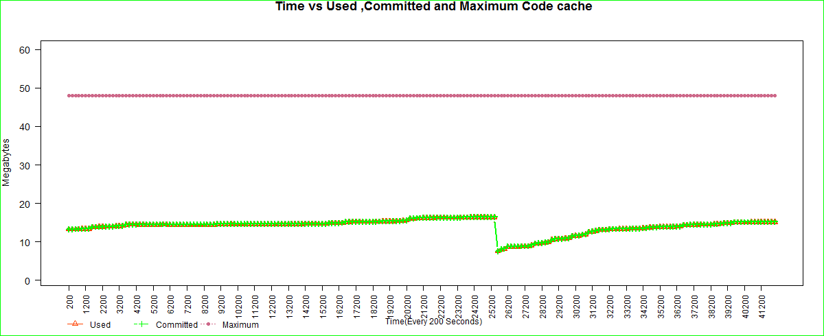
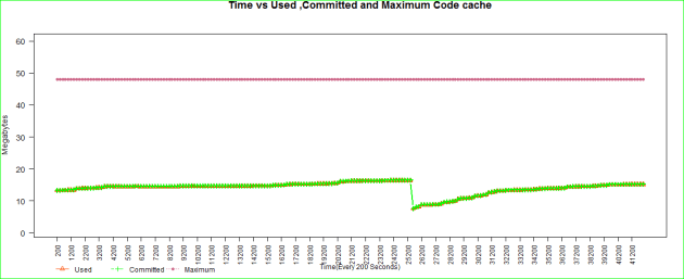
 png(
"code-cache.png",
width =1200, height = 490)


plot(data$Time,as.numeric(data$Used),ylim=c(1,60),col="orangered",pch=2,type="b", ylab="Megabytes", xlab="",las=2,lwd=2,xaxt="n", cex.lab=1.2,cex.axis=1.2)
axis(1,at = seq(min(data$Time), max(data$Time), by=1000),las = 2,cex.axis=1)

par(mar=c(5,5.5,1,1))
par(oma=c(0,0,0,0) )
box("figure",lty="solid", col="green")

title("Time vs Used ,Committed and Maximum Code cache",cex.main=1.5,xlab="Time(Every 200 Seconds)")

points(data$Time,as.numeric(data$Committed),col="green",pch=3,lwd=2, cex.lab=1.2,cex.axis=1,type="b")
points(data$Time,as.numeric(data$Max),col="palevioletred3",pch=16,lwd=2, cex.lab=1.2,cex.axis=1,type="b")

par(xpd=TRUE)
 legend(3.8,-9,c("Used", "Committed", "Maximum"), pch = c(2,3,16), lty = c(1,2,3),col=c('orangered','green','palevioletred3'),ncol=3,bty ="n")

dev.off()

The Committed and Used graph lines are together because the data is almost the same. There are some lines of ‘R’ code that are from the forums. In fact some lines related to graph layout may not be required. I always find it difficult to layout the graph. In this case the legend is at the bottom and finding space for it was hard.

When I started exploring this aspect of the JVM memory pool I was not aware that one could dump the current memory pool utilization data like this.

Kirk Pepperdine(jClarity) pointed out that he has a VisualVM plugin(https://java.net/projects/memorypoolview/) to look at JVM memory pools.

‘R’ regex

My Java Virtual Machine memory pool dump is this. I had earlier isolated only Code Cache memory pool for analysis and that is the following section. I converted this to data frame first.

1            Peak Usage    : init:2359296, used:13914944, committed:13959168, max:50331648Current Usage : init:2359296, used:13913536, committed:13959168, max:50331648|------------------| committed:13.31Mb+---------------------------------------------------------------------+|//////////////////|                                                  | max:48Mb+---------------------------------------------------------------------+|------------------| used:13.27Mb
2            Peak Usage    : init:2359296, used:13916608, committed:13959168, max:50331648Current Usage : init:2359296, used:13915200, committed:13959168, max:50331648|------------------| committed:13.31Mb+---------------------------------------------------------------------+|//////////////////|                                                  | max:48Mb+---------------------------------------------------------------------+|------------------| used:13.27Mb
3             Peak Usage    : init:2359296, used:13949120, committed:13991936, max:50331648Current Usage : init:2359296, used:13947712, committed:13991936, max:50331648|------------------| committed:13.34Mb+---------------------------------------------------------------------+|//////////////////|                                                  | max:48Mb+---------------------------------------------------------------------+|------------------| used:13.3Mb
4            Peak Usage    : init:2359296, used:13968576, committed:13991936, max:50331648Current Usage : init:2359296, used:13956224, committed:13991936, max:50331648|------------------| committed:13.34Mb+---------------------------------------------------------------------+|//////////////////|                                                  | max:48Mb+---------------------------------------------------------------------+|------------------| used:13.31Mb

I tried this to cut only Current Usage statistics. The regex is

greedy

and matches upto the first ‘pipe’ character.

y <- apply( y, 1, function(z) str_extract(z,"Current.*?[/|]"))

  [1] "Current Usage : init:2359296, used:13913536, committed:13959168, max:50331648|"
  [2] "Current Usage : init:2359296, used:13915200, committed:13959168, max:50331648|"
  [3] "Current Usage : init:2359296, used:13947712, committed:13991936, max:50331648|"
  [4] "Current Usage : init:2359296, used:13956224, committed:13991936, max:50331648|"

R users’ list member Arun recommends this

> as.matrix(gsub("^.*(Current.*?[/|]).*","\\1",y$y))

       [,1]                                                                            
  [1,] "Current Usage : init:2359296, used:13913536, committed:13959168, max:50331648|"
  [2,] "Current Usage : init:2359296, used:13915200, committed:13959168, max:50331648|"
  [3,] "Current Usage : init:2359296, used:13947712, committed:13991936, max:50331648|"
  [4,] "Current Usage : init:2359296, used:13956224, committed:13991936, max:50331648|"
  [5,] "Current Usage : init:2359296, used:13968832, committed:14024704, max:50331648|"

Both work as expected.

Average memory utilization of httpd process

I drew a graph showing the average memory utilization of a httpd process. I am not claiming that this is a rigorous approach but I get average figures over a period of time. I don’t have time in the axes because it was not needed.

library(stringr)

this.dir setwd(this.dir)
png(file="httpdaveragememory.png",width=900,height=350,res=72)

input 6.2 httpd (18)
 4.0 httpd (11)
 4.0 httpd (11)
 3.3 httpd (9)
 4.2 httpd (12)
 4.2 httpd (12)
 4.2 httpd (12)
 4.2 httpd (12)
 4.2 httpd (12)
"))

data colnames(data) data["Average"] <- "NA"
data$Average plot(row(data)[,1], data$Average,xlim=c(0,nrow(data)),col="green",pch=16,type="b", ylab="MBytes", xlab="Hours",las=2,lwd=2.5,cex.axis=1)

print(data)
dev.off()

Steps followed to parse the data

> data <- read.table(text=gsub(“[()]”,””,str_trim(input[input!=””])),sep=””,header=FALSE,stringsAsFactors=FALSE)
> data
V1 V2 V3
1 6.2 httpd 18
2 4.0 httpd 11
3 4.0 httpd 11
4 3.3 httpd 9
5 4.2 httpd 12
6 4.2 httpd 12
7 4.2 httpd 12
8 4.2 httpd 12
9 4.2 httpd 12
> colnames(data) <- c(“MB”,”Process”,”Count”)
> data
MB Process Count
1 6.2 httpd 18
2 4.0 httpd 11
3 4.0 httpd 11
4 3.3 httpd 9
5 4.2 httpd 12
6 4.2 httpd 12
7 4.2 httpd 12
8 4.2 httpd 12
9 4.2 httpd 12
> data[“Average”] <- “NA”
> data
MB Process Count Average
1 6.2 httpd 18 NA
2 4.0 httpd 11 NA
3 4.0 httpd 11 NA
4 3.3 httpd 9 NA
5 4.2 httpd 12 NA
6 4.2 httpd 12 NA
7 4.2 httpd 12 NA
8 4.2 httpd 12 NA
9 4.2 httpd 12 NA
> data$Average <- data$MB / data$Count
> data
MB Process Count Average
1 6.2 httpd 18 0.3444444
2 4.0 httpd 11 0.3636364
3 4.0 httpd 11 0.3636364
4 3.3 httpd 9 0.3666667
5 4.2 httpd 12 0.3500000
6 4.2 httpd 12 0.3500000
7 4.2 httpd 12 0.3500000
8 4.2 httpd 12 0.3500000
9 4.2 httpd 12 0.3500000
> row(data)
[,1] [,2] [,3] [,4]
[1,] 1 1 1 1
[2,] 2 2 2 2
[3,] 3 3 3 3
[4,] 4 4 4 4
[5,] 5 5 5 5
[6,] 6 6 6 6
[7,] 7 7 7 7
[8,] 8 8 8 8
[9,] 9 9 9 9
> row(data)[,1]
[1] 1 2 3 4 5 6 7 8 9

Graph