Machine Learning | MindSpace

Notes about Machine Learning fundamentals

April 26, 2016 Leave a comment

I have decided to try a different tack in this post. Gradually as I learn some basic ideas about statistics and Machine Learning I will update this post with code, graphs or procedures used to configure tools. So in a few weeks I will have charted a simple course through the basic Machine Learning terrain. I hope. But these are just basic ideas to prepare oneself to read a more advanced math text.

~~To be updated …~~ I will add more details in subsequent posts.

Tools

Anaconda based on Anaconda

GraphLab based on GraphLab

ipython based on ipython

The installation process was tortuous because I work in a corporate environment.

Install GraphLab Create with Command Line

The installation is based on dato’s instructions.

Step 1: Ensure Python 2.7.x

Anaconda with Python 2.x installation didn’t complete in my Windows 7 machine due to some access restriction. It couldn’t set this version of Python as the default.
So I installed Anaconda with Python 3.x. GraphLab works with only Python 2.x

In order to create a Python 2.7 environment the command used is

conda create -n dato-env python=2.7 anaconda

This was blocked by my Virus Scanner and I had to coax our security team to update my policy settings to allow this.

Traceback (most recent call last):
File “D:\Continuum\Anaconda3.4\Scripts\conda-script.py”, line 4, in <module>
sys.exit(main())
File “D:\Continuum\Anaconda3.4\lib\site-packages\conda\cli\main.py”, line 202,
in main
args_func(args, p)
File “D:\Continuum\Anaconda3.4\lib\site-packages\conda\cli\main.py”, line 207,
in args_func
args.func(args, p)
File “D:\Continuum\Anaconda3.4\lib\site-packages\conda\cli\main_create.py”, li
ne 50, in execute
install.install(args, parser, ‘create’)
File “D:\Continuum\Anaconda3.4\lib\site-packages\conda\cli\install.py”, line 4
20, in install
plan.execute_actions(actions, index, verbose=not args.quiet)
File “D:\Continuum\Anaconda3.4\lib\site-packages\conda\plan.py”, line 502, in
execute_actions
inst.execute_instructions(plan, index, verbose)
File “D:\Continuum\Anaconda3.4\lib\site-packages\conda\instructions.py”, line
140, in execute_instructions
cmd(state, arg)
File “D:\Continuum\Anaconda3.4\lib\site-packages\conda\instructions.py”, line
55, in EXTRACT_CMD
install.extract(config.pkgs_dirs[0], arg)
File “D:\Continuum\Anaconda3.4\lib\site-packages\conda\install.py”, line 448,
in extract
t.extractall(path=path)
File “D:\Continuum\Anaconda3.4\lib\tarfile.py”, line 1980, in extractall
self.extract(tarinfo, path, set_attrs=not tarinfo.isdir())
File “D:\Continuum\Anaconda3.4\lib\tarfile.py”, line 2019, in extract
set_attrs=set_attrs)
File “D:\Continuum\Anaconda3.4\lib\tarfile.py”, line 2088, in _extract_member
self.makefile(tarinfo, targetpath)
File “D:\Continuum\Anaconda3.4\lib\tarfile.py”, line 2128, in makefile
with bltn_open(targetpath, “wb”) as target:
PermissionError: [Errno 13] Permission denied: ‘D:\\Continuum\\Anaconda3.4\\pkgs
\\python-2.7.11-4\\Lib\\pdb.doc’

The last line shown above is what I presume was blocked by the Virus scanner. When the logs were shown to the security team who updated the scanner rules.

Learning some of these topics may be difficult if we don’t read a more advanced book. So I am constrained by the lack of deep knowledge of a related math subject.

But a question like this one must be simple. Right ?

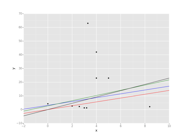
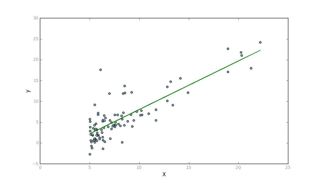
Identify which model performs better when you have the intercept, slope and Residual Sum of squares.

No data point is given.One can plot the lines when their intercepts and slopes are known but I don’t know how that helps.

Plot some lines when we know their intercepts and slopes. Data points are random though and are irrevelant at this time.

from ggplot import *
import pandas as pd
data = {'x': [0, 2, 3, 4, 5, 4, 3.2, 3.3, 2.6, 8.4],
'y': [4.2, 2.6, 1.2, 23, 23, 42, 1.2, 63, 2.3, 2.1],
}
df = pd.DataFrame(data)
g = ggplot(df, aes(x='x', y='y')) + \
geom_point() + \
geom_abline(intercept=0, slope=1.4, colour=&amp;quot;red&amp;quot;) \
+ geom_abline(intercept=3.1, slope=1.4, colour=&amp;quot;blue&amp;quot;) \
+ geom_abline(intercept=2.7, slope=1.9, colour=&amp;quot;green&amp;quot;) \
+ geom_abline(intercept=0, slope=2.3, colour=&amp;quot;black&amp;quot;)
print(g)

Filed under Machine Learning, Python

Practicing Predictive Analytics using “R”

February 7, 2016 Leave a comment

I spent a Sunday on this code to answer some questions for a Coursera course. At this time this code is the norm in more than one such course. So I am just building muscle memory. I type this code and look at the result and learn what I learnt earlier.

If I don’t remember how to solve it I search but the point is that I have to be constantly in touch with “R” as well the fundamentals. My day job doesn’t let me do this. The other option is a book on Machine Learning like the one by Tom Mitchell but that takes foreover.

setwd("~/Documents/PredictiveAnalytics")

library(dplyr)  
library(ggplot2)
library(rpart)
library(tree)
library(randomForest)
library(e1071)
library(caret)


seaflow <- read.csv(file="seaflow_21min.csv",head=TRUE)
final <-filter(seaflow, pop == "synecho")
print(nrow(final))
print( summary(seaflow))


print ( nrow(seaflow))

print( head(seaflow))

set.seed(555)
trainIndex <- createDataPartition( seaflow$file_id, p = 0.5, list=FALSE, times=1)
train <- seaflow[ trainIndex,]
test <- seaflow[ -trainIndex,]



print(mean(train$time))

p <- ggplot( seaflow, aes( pe, chl_small, color = pop)) + geom_point()
dev.new(width=15, height=14)
print(p)
ggsave("~/predictiveanalytics.png", width=4, height=4, dpi=100)
fol <- formula(pop ~ fsc_small + fsc_perp + fsc_big + pe + chl_big + chl_small)
model <- rpart(fol, method="class", data=train)
print(model)
#plot(model)
#text(model, use.n = TRUE, all=TRUE, cex=0.9)

testprediction <- predict( model, newdata=test, type="class")
comparisonofpredictions <- testprediction == test$pop
accuracy <- sum(comparisonofpredictions) / length(comparisonofpredictions)

print( accuracy )

randomforestmodel <- randomForest( fol, data = train)
print(randomforestmodel)

testpredictionusingrandomforest <- predict( randomforestmodel, newdata=test, type="class")
comparisonofpredictions <- testpredictionusingrandomforest == test$pop
accuracy <- sum(comparisonofpredictions) / length(comparisonofpredictions)
print( accuracy )

print(importance(randomforestmodel))

svmmodel <- svm( fol, data = train)

testpredictionusingsvm <- predict( svmmodel, newdata=test, type="class")
comparisonofpredictions <- testpredictionusingsvm == test$pop
accuracy <- sum(comparisonofpredictions) / length(comparisonofpredictions)
print( accuracy )

predictiveanalytics

Filed under Machine Learning, R

Microsoft: Data Science and Machine Learning Essentials

October 23, 2015 2 Comments

After completing this edX course successfully I identified these questions which I answered wrongly. In some cases I selected more than the required options due to oversight.

~~I have marked the likely answers.~~

I need a longer article to explain what I learnt which I plan to write soon.

You have amassed a large volume of customer data, and want to determine if it is possible to identify distinct categories of customer based on similar characteristics.

What kind of predictive model should you create?

1. Regression
2. Clustering
3. Recommender
4. Classification

You discover that there are missing values for an unordered numeric column in your data.
Which three approaches can you consider using to treat the missing values?

1. Substitute the text “None”.
2. Forward fill or back fill the value.
3. Remove rows in which the value is missing.
4. Interpolate a value to replace the missing value.
5. Substitute the numeral 0

When assessing the residuals of a regression model you observe the following:

Residuals exhibit a persistent structure and are not randomly distributed with respect to values of the label or the features.
The Q-Q normal plots of the residuals show significant curvature and the presence of outliers.
Given these results, which two of the following things should you try to improve the model?

1. Cross validate the model to ensure that it will generalize properly.
2. Try a different class of regression model that might better fit the problem should be tried.
3. Create some engineered features with behaviors more closely tracking the values of the label.
4. Add a Sweep Parameters module with the Metric for measuring performance for classification property set to Accuracy.

You create an experiment that uses a Train Matchbox Recommender module to train a recommendation model, and add a Score Matchbox Recommender module to generate a prediction. You want to use the model in a music streaming service to recommend songs for the currently logged in user.Which recommender prediction kind should you configure the Score Matchbox

Recommender module to use?

1. Item Recommendation
2. Related Items
3. Rating Prediction
4. Related Users

While exploring a dataset you discover a nonlinear relationship between certain features and the label.Which two of the following feature engineering steps should you try before training a supervised machine learning model?

1. Ensure the features are linearly independent.
2. Compute new features based on polynomial values of the original features.
3. Compute mathematical combinations of the label and other features.
4. Compute new features based on logarithms or exponentiation of these original features.

Which two of the following approaches can you use to determine which features to prune in an Azure ML experiment?

1. Use the Permutation Feature Importance model to identify features of near-zero importance.
2. Use the Cross Validation module to identify folds which indicate the model does not generalize well.
3. Prune features one at a time to find features which reduce model performance or have no impact on model performance as measured with the Evaluate Model module.
4. Use the Split module to create training, test and evaluation data sub-sets to evaluate model performance.

Filed under Azure ML, Machine Learning

Gradient Descent

October 6, 2015 Leave a comment

I ported the Gradient Descent code from Octave to Python. The base Octave code is the one from Andrew Ng’s Machine Learning MOOC.

I mistakenly believed that the Octave code for matrix multiplication will directly translate in Python.

The matrices are these.

But the Octave code is this

Octave code

  theta = theta - ( (  alpha * ( (( theta' * X' )' - y)' * X ))/length(y) )'

and the Python code is this.

Python

def gradientDescent( X,
                     y,
                     theta,
                     alpha = 0.01,
                     num_iters = 1500):

    r,c = X.shape
    
    for iter in range( 1, num_iters ):
        theta = theta - ( ( alpha * np.dot( X.T, ( np.dot( X , theta ).T - np.asarray(y) ).T ) ) / r )
    return theta

This line is not a direct transalation.

        theta = theta - ( ( alpha * np.dot( X.T, ( np.dot( X , theta ).T - np.asarray(y) ).T ) ) / r )

But only the above Python code gives me the correct theta that matches the value given by the Octave code.

Linear Regression

But the gradient descent also does not give me the correct value after a certain number of iterations. But the cost value is similar.

Gradient Descent from Octave Code that converges

Minimization of cost

Initial cost is 640.125590
J = 656.25
Initial cost is 656.250475
J = 672.58
Initial cost is 672.583001
J = 689.12
Initial cost is 689.123170
J = 705.87
Initial cost is 705.870980
J = 722.83
Initial cost is 722.826433
J = 739.99
Initial cost is 739.989527

Gradient Descent from my Python Code that does not converge to the optimal value

Minimization of cost

635.81837438
651.963633303
668.316534159
684.877076945
701.645261664
718.621088313
735.804556895

Filed under Machine Learning, Python

Azure Machine Learning

October 4, 2015 Leave a comment

The AzureML Studio user interface is slick, very responsive and adopts a workflow supporting both R and Python scripts. There is a free account available with this caveat but that did not hamper my efforts to test some simple flows.

Note: Your free-tier Azure ML account allows you unlimited access, with some reduced capabilities compared to a full Microsoft Azure subscription. Your experiments will only run at low priority on a single processor core. As a result, you will experience some longer wait times. However, you have full access to all features of Azure ML.

The graph visualizations are very spiffy too. I am yet to finish the data cleansing aspects and use the really interesting ML algorithms.

Filed under Azure ML, Machine Learning

Principal Component Analysis

September 28, 2015 Leave a comment

This is about what I think I understood about Principal Component Analysis. I will update this blog post later.

The code is in github and it works but I think the eigen values could be wrong. I have to test it further.

These are the two main functions.


    """Compute the covariance matrix for a given dataset.
    """
def estimateCovariance( data ):
    print data
    mean = getmean( data )
    print mean
    dataZeroMean = map(lambda x : x - mean, data )
    print dataZeroMean
    covar = map( lambda x : np.outer(x,x) , dataZeroMean )
    print getmean( covar ) 
    return getmean( covar )

    """Computes the top `k` principal components, corresponding scores, and all eigenvalues.
    """
def pca(data, k=2):
    
    d = estimateCovariance(  data )
    
    eigVals, eigVecs = eigh(d)

    validate( eigVals, eigVecs )
    inds = np.argsort(eigVals)[::-1]
    topComponent = eigVecs[:,inds[:k]]
    print '\nTop Component: \n{0}'.format(topComponent)
    
    correlatedDataScores = map(lambda x : np.dot( x ,topComponent), data )
    print ('\nScores : \n{0}'
       .format('\n'.join(map(str, correlatedDataScores))))
    print '\n eigenvalues: \n{0}'.format(eigVals[inds])
    return topComponent,correlatedDataScores,eigVals[inds]

Filed under Machine Learning, PCA, Python

Deep learning course at the University of Oxford.: 2014-2015 and another MIT book

May 19, 2015 Leave a comment

I am viewing these Course materials with a feeling of awe. I hope these resources provide some fodder for this blog and my imagination.

One more.

An MIT Press book in preparation

Yoshua Bengio, Ian Goodfellow and Aaron Courville

DEEP LEARNING

One more.

The wonderful resources by Andrej Karpathy

Filed under Machine Learning

sigmoid function

March 22, 2015 Leave a comment

What is a sigmoid function ?

It is http://mathworld.wolfram.com/SigmoidFunction.html

This simple code is the standard way to plot it. I am using Octave.

x = -10:0.1:10;
a = 1.0 ./ (1.0 + exp(-x));
figure;
plot(x,a,'-','linewidth',3)

Filed under Machine Learning, R

The Caltech-JPL Summer School on Big Data Analytics

October 13, 2014 Leave a comment

This treasure trove of videos teach many Machine Learning subjects. This is not intended to be a typical Coursera course because there are no deadlines or tests.

There is so much to write about what I learn from these videos but for now these measures to assess the costs and benefits of a classification model are intended as reference.