Streams

I tried to use lambdas to swap elements in the char[] array. Does this mean that I am trying to change the stream while it is streaming ? This code is from http://www.cs.uofs.edu/~mccloske/courses/cmps144/invariants_lec.html but this question is unrelated to those concepts.

If that is a problem then a new stream will do. How should this be done ? I am not looking for a Comparator. I would like to work with this code as it is without using any API but lambdas.

I am printing using lambdas in this code now.

public class DutchNationalFlag {

    private static final int N = 10;

    private static char[] flags = new char[]{'R','B','B','R','R','B','B','R','R','B'};

    public static void main( String... argv){

        new String(flags).chars().mapToObj(i -> (char)i).forEach(System.out::println);

        int m = 0,  k = 0;
        while (m != N)  {
            if (flags[m] == 'B') { }
            else {
                swap(flags,k,m); 
                k = k+1;
            }
            m = m+1;
        } 
        new String(flags).chars().mapToObj(i -> (char)i).forEach(System.out::println);
    }

    private static void swap(char[] flags, int k, int m) {

        char temp = flags[k];
        flags[k] = flags[m];
        flags[m] =  temp;

    }

}

Possible Solution 1:

This doesn’t do exactly what the original code does. It doesn’t swap and doesn’t advance k which is the boundary between ‘B’ and ‘R’.But it produces the result.

    Stream<Character> stream1 = 
    IntStream.range(0, flags.length).mapToObj(i -> (char)flags[i]);

    Stream<Character> stream2 = 
    IntStream.range(0, flags.length).mapToObj(i -> (char)flags[i]);


    Stream.concat(stream2.filter(x-> (x == 'B')), stream1.filter( y->(y == 'R')  )).forEach(System.out::println);
Steve Vinoski recommends these papers

One does not need a degree from the IIT  to read and understand these papers. These are accessible and one has to persevere. That is all. In India technical work is considered taboo because the society thinks it is the prerogative of people with advanced degrees.

Steve Vinoski recommends these papers.


“Eventual Consistency Today: Limitations, Extensions, and Beyond”, Peter Bailis, Ali Ghodsi. This article provides an excellent description of eventual consistency and
recent work on eventually consistent systems.

“A comprehensive study of Convergent and Commutative Replicated Data Types”, M. Shapiro, N. Preguiça, C. Baquero, M. Zawirski. This paper explores and details data types that work well for applications built on eventually consistent systems.

“Notes on Distributed Systems for Young Bloods”, J. Hodges. This excellent blog post succinctly summarizes the past few decades of
distributed systems research and discoveries, and also explains some implementation concerns we’ve learned along the way to keep in mind when build distributed applications.

“Impossibility of Distributed Consensus with One Faulty Process”, M.Fischer, N. Lynch, M. Paterson. This paper is nearly 30 years old but is critical to understanding fundamental properties of distributed systems.

“Dynamo: Amazon’s Highly Available Key-value Store”, G. DeCandia, et al. A classic paper detailing trade-offs for high availability distributed systems.

rJava, rCharts and R code to display GC data

These are the steps I follow to display GC activity data using a nvd3 discrete bar chart.

Call Java class using rJava

  gctypes <- .jcall(realtimegcdataobserver ,"Ljava/util/List;","getGCTypes")

Create an empty data frame to hold the data

I get the type of the GC algorithm, GC count and time from JMX. I have yet to explore the last two values.

gcdata <- function(){
  df <- data.frame(
                 GCType=character(), 
                 Count=character(),
                 Time=character(), 
                 stringsAsFactors=FALSE)
  print(df)
  return(df)
}

Iterate over the list of beans

Call appropriate methods and fill up the empty data frame.
I massage the data using the last two lines but don’t know any elegant way to accomplish this.

  emptygcdata <- gcdata()
  gctypedetails <- sapply( gctypes, function(item) rbind(emptygcdata, as.data.frame(c(GCType=item$getName(),Count=item$getL(),Time=item$getM()))))

  gctypedetails <- data.frame(gctypedetails)
  gctypedetails <- data.frame(matrix(unlist(gctypedetails)))

matrix.unlist.gctypedetails..
1 PS Scavenge
2 16
3 22
4 PS MarkSweep
5 0
6 0


emptygcdata <- gcdata()
  before <- 0
  after <- 2
  repeat
  {
    if (after >= nrow(gctypedetails))
     break;
    emptygcdata <- rbind(emptygcdata, data.frame(GCType =gctypedetails[before + 1,1], Count =gctypedetails[before + 2,1], Time=gctypedetails[before + 3,1]))
    before <- after + 1;
    after <- after + 2;
   }

 GCType          Count  Time
1  PS Scavenge      16  22
2  PS MarkSweep     0  0

nvd3 using rCharts

  p2 = nPlot(x = "Time", y = "Count", data = emptygcdata, type = "discreteBarChart")
  p2$chart(
    color = "#! function(d){
      var ourColorScale = d3.scale.ordinal().domain(['PS MarkSweep','PS Scavenge']).range(['green','purple']);
      return ourColorScale(d.GCType);
    }!#")

Varargs

Is this confusing code ? I was stumped for a few seconds.

public class PassThreeValues {
     static void calculateSomeThing(int one, int... values){}

     public static void main( String... argv ){                 
         calculateSomeThing(1,2,3);
    }

‘R’ and Java Lambda

> head(y)
                                                                                                                                                                                                                                                                                                                                                                                                                                                              y
1 Peak Usage    : init:2359296, used:13914944, committed:13959168, max:50331648Current Usage : init:2359296, used:13913536, committed:13959168, max:50331648|------------------| committed:13.31Mb+---------------------------------------------------------------------+|//////////////////|                                                  | max:48Mb+---------------------------------------------------------------------+|------------------| used:13.27Mb
> y <- apply( y, 1, function(z) str_extract(z,"Current.*?[/|]"))
[1] "Current Usage : init:2359296, used:13913536, committed:13959168, max:50331648|"

The ‘R’ function ‘apply’ can operate on a data structure and apply a regular expression. It gives back a data structure with the new values.

I think the equivalent Java Lambda code could be like this. It may not be optimal but the result is similar.


import java.util.ArrayList;
import java.util.List;
import java.util.regex.Matcher;
import java.util.regex.Pattern;
import java.util.stream.Collectors;


public class ArrayListStream {

    public static void main( String... argv ){
        List<String> list = new ArrayList();
        list.add( "Peak Usage    : init:2359296, used:13914944, committed:13959168, max:50331648Current Usage : init:2359296, used:13913536, committed:13959168, max:50331648|------------------| committed:13.31Mb+---------------------------------------------------------------------+|//////////////////|                                                  | max:48Mb+---------------------------------------------------------------------+|------------------| used:13.27Mb");
        list.add( "Peak Usage    : init:2359296, used:13916608, committed:13959168, max:50331648Current Usage : init:2359296, used:13915200, committed:13959168, max:50331648|------------------| committed:13.31Mb+---------------------------------------------------------------------+|//////////////////|                                                  | max:48Mb+---------------------------------------------------------------------+|------------------| used:13.27Mb");
        Pattern p = Pattern.compile( "Current.*?[/|]" );
        List list1 = list.
                       stream().
                        map(p::matcher).
                          filter(Matcher::find).map(matcher -> matcher.group()).
                              collect(Collectors.toCollection(ArrayList::new));
        System.out.println(list1.get(0));
    }
}

”R” code kata

This started as a ‘R’ code kata. I came across some Nmon reports from a AIX machine.

There is an nmon analyzer too available in IBM’s website.

The goal here is to learn to write ‘R’ code to ‘grep’ for lines that have information for CPU’s like this

CPU01,T0001,7.6,28.9,1.3,62.1
CPU02,T0001,4.9,6.5,1.1,87.5
CPU03,T0001,2.4,2.1,0.4,95.1
CPU04,T0001,2.9,1.4,0.8,94.9

Not only that. I also want to draw graphs for individual CPU’s and find if there are correlations between different CPU utilizations. This type of analysis is described in some papers published by ‘Computer Measurement Group’. I don’t have the links now but I plan to post more about this along with the graphs.

At this time this is not a serious performance planning measure. But it should be possible to use ‘R’ code to create a good nmon analyzer report.

This initial version of the code executes but it is not complete.

YAML configuration

path:
 input : D:\R\R-3.0.0\bin\MACHINE_130525_0000.csv
 output : D:\R\R-3.0.0\bin

Main code


library(yaml)
library(stringr)

# Set to load the configuration file.
# It might be set elsewhere also.
this.dir <- dirname(parent.frame(2)$ofile) 
setwd(this.dir) 

# Read nmon report and filter CPU utilization
filelist.read <- function(){
	config = yaml.load_file("config.yml")
	print(config$path$input)
	output <-(config$path$output)
	nmon <-file(config$path$input, "r")
	fileConn<-file(paste(output,"\\output.txt", sep = ""),"w")

	files <- NULL

	while(length(line <- readLines(nmon, 1)) > 0) {
		files <- line.filter( line )
		if (length(files) != 0) {
			writeLines(files, fileConn)
			#print(files)
			files <- NULL
		}
	}
	close(nmon)
	close(fileConn)
}

#filter based on a regular expression
line.filter <- function(line){
	filteredline <- grep("^CPU", line, value = TRUE)
	return (filteredline)
}


#Write each CPU's utilization data into a 
#separate file
filelist.array <- function(n){
  cpufile <- list()
  length(cpufile) <- n
  for (i in 1:n) {
    cpufile[[i]] <- paste("output", i, ".txt", sep = "") 
    print(cpufile[i])	
  }
}
#Write each CPU's utilization into a 
#separate file
filelist.array <- function(n){
         cpufile <- list()
         length(cpufile) <- n
         for (i in 1:n) {
            cpufile[[i]] <- paste("output", i, sep = "")
            print(cpufile[i])
         }
}

RUnit

library(RUnit)

#Sample test
test.filelist.array <- function() {
	filelist.array(3)
}

RUnit test runner

library(RUnit)

# Set to load sources and test code
# properly.
this.dir <- dirname(parent.frame(2)$ofile) 
setwd(this.dir) 

source('nmon.R')
source('unitTests/nmontestcase.R')
test.filelist.array()

Graph model

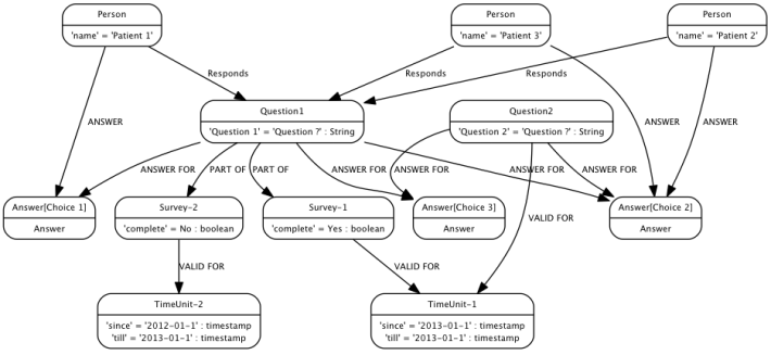
Deliver an online site where patients can view and respond to a series of questions that help to determine their eligibility for a clinical trials*. A patient should be able to save their data and come back at a later date to update or complete the survey. 

I was asked to draw a model for surveys recently. The surveys have questions and answers. A few years back I worked on a system that popped up questions in order to diagnose problems reported by customers. So based on the answers new questions will be posed on a site to enable diagnosis. So at that time we used a RDBMS and it did not seem to be a natural way of representing complex branches of questions and answers.

Now I realize a graph model represented in Neo4J graph DB can be a more flexible model. So a graph looks like a more realistic model of a survey.


  1. A proper model matching the problem
  2. Versioning and storage of historical records of entire surveys are possible
  3. Querying for historical records based on timestamped versions is possible. In this case ‘TimeUnit’ can be shown as a first-class graph node and not just data in a RDBMS.
  4. Reusability of answers and questions are clearly represented.

I am neither a RDBMS expert or a graph expert but the model shown below seems flexible enough.

Image


Weaving java.util.concurrent API using AspectJ

I stopped using AspectJ long back because we were not really coding aspects because it required an enormous amount of effort to train others. But recently I wrote this to weave into java.util.concurrent libraries to try to explore how the ForkJoin library works. Even though the code works I thought it is not a recommended way to weave into libraries dealing with concurrency written by experts. I pulled  the source and created a custom JAR and used -Xbootclasspath to make it work.


@Aspect
public class ForkJoinProjector {


    @Pointcut( "execution ( int java.util.concurrent.ForkJoinPool.registerWorker(java.util.concurrent.ForkJoinWorkerThread)) &&" +
			                " args(thread) &&" +
			                " target(pool)" )
    public void buildQueues( ForkJoinWorkerThread thread,
	                     ForkJoinPool pool){}
	
    @After("buildQueues( thread,pool)")
    public void build( ForkJoinWorkerThread thread,
    		           ForkJoinPool pool ) {
    	System.out.println( "ID " + thread.getId() + " Name " + thread.getName() );
    }


}

The Alan Turing Year

Image

I am watching the UEFA match between Poland and Greece and ruing the lack of professional ethics in the project management community and the great divide that exists between them and the technical team and I came across The Alan Turing Year. There is a flood of information here.

Rising stars or shooting stars

I have lamented in the past about organization structures in India that promote people to dizzying heights in a short span of time. These people are the ‘rising stars’ and they never gain expertise in any field. They pick a plum technical project to work on so that the next appraisal process favors them not because they are experts but because they are part of a highly visible team that boosted the financial success of the firm.

This is from ‘The Five stages of Capacity Planning’ by H Pat Artis

“Because capacity planning in this stage is a high visibility special project, it is often assigned to rising stars who will have long since been promoted by the time of the next planning cycle occurs.”

These rising stars are shooting stars who do not continue as technical leads and a newer crop of junior people take their place leading to standards that fall precipitously.