R | MindSpace | Page 2

Gram-schmidt

November 4, 2014 Leave a comment

Matrix M has three rows and three columns, and the columns form an orthonormal basis. One of the columns is [2/7,3/7,6/7], and another is [6/7, 2/7, -3/7]. Let the third column be [x,y,z]. Since the length of the vector [x,y,z] must be 1, there is a constraint that x2+y2+z2 = 1. However, there are other constraints, and these other constraints can be used to deduce facts about the ratios among x, y, and z. Compute these ratios, and then identify one of them in the list below.

I viewed the Khan academy course.

But the credit for the Matlab code goes to Vladd. I didn’t follow his explanation but the Khan academy course helped.I used the Matlab online compiler to test Vladd’s code and ported it to R.

I can’t believe the for and if loops in the R code took a full day to debug.


# TODO: Add comment
# 
# Author: radhakrishnan
###############################################################################


        A =  matrix(c(2/7,3/7,6/7,6/7,2/7,-3/7,1,2,3),ncol=3,nrow=3)
		r = dim( A)[[1]];
		c = dim( A)[[2]];
		print(A)
		
		Q = matrix(c(0,0,0,0,0,0,0,0,0),ncol=3,nrow=3)
		for (j in 1:3){

			u = matrix(A[ ,j  ]);
	
			if( j - 1 != 0 ){
				for(i in 1:(j - 1)){
				    e = Q[,i]
					a = as.matrix(A[,j])
					p = (t(e) %*% a) / (t(e) %*% e) * e;
					u = u - p
		        }
			}
           # normalize it to length of 1 and store it
			Q[,j] = u / sqrt(u[1,1]^2 + u[2,1]^2 + u[3,1]^2);
			print(Q)
		}

The result is this. The last column is what I want and that satisfies all constraints.

Orthonormality

$\begin{pmatrix} 0.2857143& 0.8571429& -0.4285714\\ 0.4285714& -0.2857143& 0.8571429\\ 0.8571429& -0.4285714& -0.2857143\\ \end{pmatrix}$

I will check-in the R code into my Git repository.

Filed under Data Mining Algorithms, R

Market-basket problem

October 18, 2014 Leave a comment

This is the general market-basket problem. It is an algorithm to find how many items are frequently found across many shoppers’ baskets based on a threshold. The threshold is a minimum number of occurrences of a particular item. Items that are bought a certain number of times(threshold) are considered frequent.

These items can be singletons or pairs of items(doubletons) and tripletons and so on.

Imagine there are 100 baskets, numbered 1,2,...,100, and 100 items, similarly numbered. Item i is in basket j if and only if i divides j evenly. For example, basket 24 is the set of items {1,2,3,4,6,8,12,24}. Describe all the association rules that have 100% confidence. Which of the following rules has 100% confidence?

A brute-force R approach to solve such a problem. This is a small number of items. In fact such data mining algorithms deal with large quantities of data and a fixed amount of memory. One such algorithm is the A-priori algorithm.

Each of the if loop checks for a condition like this.

 {8,10} -> 20

This checks if item 20 is always found in a basket that has items 8 and 10 or not.

library(Hmisc)
for( i in 1:100){
  a <- 1
  for( j in 1:100){

	if( i %% j == 0 ){
		a <- append(a,j)
        }
  }
  #print(paste( i, a ))
  if( 8 %in% a &&  10 %in% a && 20 %nin% a ){ //{8,10} -> 20
	#print (a)
  }
  if( 3 %in% a &&  1 %in% a && 6 %in% a && 12 %nin% a ){
	print (a)
  }
  if( 8 %in% a &&  12 %in% a &&  96 %nin% a ){
	#print (a)
  }
  if( 3 %in% a &&  5 %in% a &&  1 %nin% a ){
	#print (a)
  }
}}

Filed under Data Mining Algorithms, R

PageRank

October 4, 2014 2 Comments

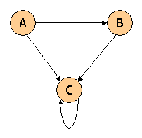
Suppose we compute PageRank with a β of 0.7, and we introduce the additional constraint that the sum of the PageRanks of the three pages must be 3, to handle the problem that otherwise any multiple of a solution will also be a solution. Compute the PageRanks a, b, and c of the three pages A, B, and C, respectively.

$A = \sum_{i\rightarrow{j}} \beta r_i/d_i + (1 - \beta ) e / n$

My R code is this.

M = matrix(c(0,1/2,1/2,0,0,1,0,0,1),ncol=3)
e = matrix(c(1,1,1),ncol=1)
v1 = matrix(c(1,1,1),ncol=1) 
v1 = v1 / 3
for( i in 1:5){

  v1 =  ((0.7 * M ) %*% v1 ) + (((1 - 0.7 ) * e ) /3 )
}
   v1 = v1 * 3

      [,1]
[1,] 0.300
[2,] 0.405
[3,] 2.295

Filed under R

Apache Mahout

September 29, 2014 Leave a comment

I followed this tutorial. Mahout seems to be an easy way to test Machine Learning algorithms using the Java API.

But I would use this this R code instead of the one shown in the tutorial to convert the MovieLens dataset to CSV format.

r<-file("u.data","r")
w<-file("u1.csv","w")

while( length(data <- readLines(r)) > 0 ){
	writeLines(gsub("\\s+",",",data),w)
}

Filed under Machine Learning, R

Time series forecast

September 27, 2014 Leave a comment

This code counts how many values from the testing dataset fall within the 95% Confidence Interval range.

library(forecast)
library(lubridate)  # For year() function below
dat=read.csv("~/Desktop/gaData.csv")
training = dat[year(dat$date) < 2012,]
testing = dat[(year(dat$date)) > 2011,]
tstrain = ts(training$visitsTumblr)
sum <- 0
 fit <- bats(tstrain)
 fc <- forecast(fit,h=235)
 mat <- fc$upper
 for(i in 1:nrow(mat)){
     v <- data.frame(mat[i,])
     print(paste(testing$visitsTumblr[i],v[1,] , v[2,]))
     if(testing$visitsTumblr[i] > v[1,] & testing$visitsTumblr[i] < v[2,]){
	sum <- sum + 1
     }
 }
     print(sum)

The forecast object has this type of data(Lo 95 & Hi 95) which I use.

> fc
    Point Forecast     Lo 80    Hi 80     Lo 95    Hi 95
366       207.4397 -124.2019 539.0813 -299.7624 714.6418
367       197.2773 -149.6631 544.2177 -333.3223 727.8769
368       235.5405 -112.0582 583.1392 -296.0658 767.1468
369       235.5405 -112.7152 583.7962 -297.0707 768.1516
370       235.5405 -113.3710 584.4520 -298.0736 769.1546
371       235.5405 -114.0256 585.1065 -299.0747 770.1556
372       235.5405 -114.6789 585.7599 -300.0739 771.1548

Filed under Machine Learning, R

Lasso fit

September 26, 2014 Leave a comment

The code I was given

set.seed(3523)
library(AppliedPredictiveModeling)
data(concrete)
inTrain = createDataPartition(concrete$CompressiveStrength, p = 3/4)[[1]]
training = concrete[ inTrain,]
testing = concrete[-inTrain,]

This is the data

<- head(as.matrix(training))
    Cement BlastFurnaceSlag FlyAsh Water Superplasticizer CoarseAggregate
47   349.0              0.0      0 192.0              0.0          1047.0
55   139.6            209.4      0 192.0              0.0          1047.0
56   198.6            132.4      0 192.0              0.0           978.4
58   198.6            132.4      0 192.0              0.0           978.4
63   310.0              0.0      0 192.0              0.0           971.0
115  362.6            189.0      0 164.9             11.6           944.7
    FineAggregate Age CompressiveStrength
47          806.9   3               15.05
55          806.9   7               14.59
56          825.5   7               14.64
58          825.5   3                9.13
63          850.6   3                9.87
115         755.8   7               22.90

Lasso fit and plot

predictors <- as.matrix(training)[,-9]
lasso.fit <- lars(predictors,training$CompressiveStrength,type="lasso",trace=TRUE)
headings <- names(training[-(9:10)])
plot(lasso.fit, breaks=FALSE)
legend("topleft", headings,pch=8, lty=1:length(headings),col=1:length(headings))

According to this graph the last coefficient to be set to zero as the penalty increases is Cement. I think this is correct but I may change this.

Filed under Machine Learning, R

RandomForests

September 22, 2014 Leave a comment

I am just posting R code at this time. The explanation is missing but I am making some progress.

library(ElemStatLearn)
library(randomForest)
data(vowel.train)
data(vowel.test)

> head(vowel.train)
y x.1 x.2 x.3 x.4 x.5 x.6 x.7 x.8 x.9 x.10
1 1 -3.639 0.418 -0.670 1.779 -0.168 1.627 -0.388 0.529 -0.874 -0.814
2 2 -3.327 0.496 -0.694 1.365 -0.265 1.933 -0.363 0.510 -0.621 -0.488
3 3 -2.120 0.894 -1.576 0.147 -0.707 1.559 -0.579 0.676 -0.809 -0.049
4 4 -2.287 1.809 -1.498 1.012 -1.053 1.060 -0.567 0.235 -0.091 -0.795
5 5 -2.598 1.938 -0.846 1.062 -1.633 0.764 0.394 -0.150 0.277 -0.396
6 6 -2.852 1.914 -0.755 0.825 -1.588 0.855 0.217 -0.246 0.238 -0.365

vowel.train$y <- factor(vowel.train$y)
set.seed(33833)
fit.rf <- randomForest(vowel.train$y ~ .,data=vowel.train)
plot(fit.rf)
varImpPlot(fit.rf)

I was asked to find the order of variable importance which this graph shows.

Filed under Machine Learning, R

Principal Component Analysis

September 18, 2014 Leave a comment

library(caret)
library(AppliedPredictiveModeling)
set.seed(3433)
data(AlzheimerDisease)
adData = data.frame(diagnosis,predictors)
inTrain = createDataPartition(adData$diagnosis, p = 3/4)[[1]]
training = adData[ inTrain,]
testing = adData[-inTrain,]

I recently studied Predictive Analytics techniques as part of a course. I was given the code shown above. I generated the following two predictive models to compare their accuracy figures. This might be easy for experts but I found it tricky. So I post the code here for my reference.

Non-PCA

training1 <- training[,grepl("^IL|^diagnosis",names(training))]

 test1 <- testing[,grepl("^IL|^diagnosis",names(testing))]

 modelFit <- train(diagnosis ~ .,method="glm",data=training1)

 confusionMatrix(test1$diagnosis,predict(modelFit, test1))

Confusion Matrix and Statistics

Reference

Prediction Impaired Control

Impaired 2 20

Control 9 51

Accuracy : 0.6463

95% CI : (0.533, 0.7488)

No Information Rate : 0.8659

P-Value [Acc > NIR] : 1.00000

Kappa : -0.0702

Mcnemar’s Test P-Value : 0.06332

Sensitivity : 0.18182

Specificity : 0.71831

Pos Pred Value : 0.09091

Neg Pred Value : 0.85000

Prevalence : 0.13415

Detection Rate : 0.02439

Detection Prevalence : 0.26829

Balanced Accuracy : 0.45006

‘Positive’ Class : Impaired

PCA

training2 <- training[,grepl("^IL",names(training))]

preProc <- preProcess(training2,method="pca",thresh=0.8)

test2 <- testing[,grepl("^IL",names(testing))]

trainpca <- predict(preProc, training2)

testpca <- predict(preProc, test2)

modelFitpca <- train(training1$diagnosis ~ .,method="glm",data=trainpca)

confusionMatrix(test1$diagnosis,predict(modelFitpca, testpca))

Confusion Matrix and Statistics

Reference
Prediction Impaired Control
Impaired 3 19
Control 4 56

Accuracy : 0.7195
95% CI : (0.6094, 0.8132)
No Information Rate : 0.9146
P-Value [Acc > NIR] : 1.000000

Kappa : 0.0889
Mcnemar’s Test P-Value : 0.003509

Sensitivity : 0.42857
Specificity : 0.74667
Pos Pred Value : 0.13636
Neg Pred Value : 0.93333
Prevalence : 0.08537
Detection Rate : 0.03659
Detection Prevalence : 0.26829
Balanced Accuracy : 0.58762

‘Positive’ Class : Impaired

Filed under Machine Learning, R

Open Government Data Platform India

September 14, 2014 1 Comment

I found many datasets in this site but many of them are not useful. Some of them are just junk and others are not useful for predictive analytics.

But I found one that I actually used. The y-axis labels are smudged but that can be fixed.

The data is JSON which I parsed.

library(RJSONIO)
library(ggplot2)
library(reshape2)
library(grid)
this.dir <- dirname(parent.frame(2)$ofile) 
setwd(this.dir)

airlines   = fromJSON("json")
df <- sapply(airlines$data,unlist)
df <- data.frame(t(df))
colnames(df) <- c( (airlines[[1]][[1]])[[2]], (airlines[[1]][[2]])[[2]], (airlines[[1]][[3]])[[2]], (airlines[[1]][[4]])[[2]], (airlines[[1]][[5]])[[2]], (airlines[[1]][[6]])[[2]], (airlines[[1]][[7]])[[2]], (airlines[[1]][[8]])[[2]], (airlines[[1]][[9]])[[2]],(airlines[[1]][[10]])[[2]] )

df.melted <- melt(df, id = "YEAR")
print(class(df.melted$value))
df.melted$value<-as.numeric(df.melted$value) 
df.melted$value <- format(df.melted$value, scientific = FALSE)
print(ggplot(data = df.melted, aes(x = YEAR, y = value, color = variable)) +geom_point() + theme(axis.text.x = element_text(angle = 90,hjust = 0.9))  + theme(axis.text.y = element_text(angle = 360, hjust = 1, size=7.5, vjust=1))+ theme(plot.margin =unit(c(3,1,0.5,1), "cm")) + ylab("")  + theme(legend.text=element_text(size=6)))

This is the sample data.

 head(df)
     YEAR INTERNATIONAL  ACM (IN NOS) DOMESTIC ACM (IN NOS) TOTAL ACM (IN NOS)
1 1995-96                       92515                314727             407242
2 1996-97                       94884                324462             419346
3 1997-98                       98226                317531             415757
4 1998-99                       99563                325392             424955
5 1999-00                       99701                368015             467716
6 2000-01                      103211                386575             489786
  INTERNATIONAL PAX (IN NOS) DOMESTIC PAX (IN NOS) TOTAL PAX (IN NOS)
1                   11449756              25563998           37013754
2                   12223660              24276108           36499768
3                   12782769              23848833           36631602
4                   12916788              24072631           36989419
5                   13293027              25741521           39034548
6                   14009052              28017568           42026620
  INTERNATIONAL FREIGHT (IN MT) DOMESTIC FREIGHT (IN MT) TOTAL FREIGHT (IN MT)
1                        452853                   196516                649369
2                        479088                   202122                681210
3                        488175                   217405                705580
4                        474660                   224490                699150
5                        531844                   265570                797414
6                        557772                   288373                846145

Filed under R

Decision Tree

September 4, 2014 4 Comments

This is a technique used to analyze data for prediction. I came across this when I was studying Machine Learning.

Tree models are computationally intensive techniques for recursively partitioning response variables into subsets based on their relationship to one or more (usually many) predictor variables.

> head(data)
  file_id time cell_id    d1    d2 fsc_small fsc_perp fsc_big    pe chl_small
1     203   12       1 25344 27968     34677    14944   32400  2216     28237
2     203   12       4 12960 22144     37275    20440   32400  1795     36755
3     203   12       6 21424 23008     31725    11253   32384  1901     26640
4     203   12       9  7712 14528     28744    10219   32416  1248     35392
5     203   12      11 30368 21440     28861     6101   32400 12989     23421
6     203   12      15 30032 22704     31221    13488   32400  1883     27323
  chl_big     pop
1    5072    pico
2   14224   ultra
3       0    pico
4   10704   ultra
5    5920 synecho
6    6560    pico

training <- createDataPartition(data$pop, times=1,p=.5,list=FALSE)
train <- data[training,]
test <- data[,training]

fol <- formula(pop ~ fsc_small + fsc_perp + fsc_big + pe + chl_big + chl_small)
model <- rpart(fol, method="class", data=train)
print(model)

n= 36172

node), split, n, loss, yval, (yprob)
* denotes terminal node

1) root 36172 25742 pico (0.0014 0.18 0.29 0.25 0.28)
2) pe=41300 5175 660 nano (0 0.87 0 0 0.13) *
11) chl_small=5001.5 9856 783 synecho (0.0052 0.054 0.0051 0.92 0.015)
6) chl_small>=38109.5 653 133 nano (0.078 0.8 0 0.055 0.07) *
7) chl_small< 38109.5 9203 166 synecho (0 0.0015 0.0054 0.98 0.011) *

Filed under Machine Learning, R

← Older posts

Newer posts →