Throughput and Response time curves using R

I started using ‘R’, the statistical language, recently but its power is sorely missed in the IT industry especially in the project management and Capacity planning fields. In fact rigorous data quantification and analysis is given the short shrift by us in our software management activities like calculation of schedule variance and trends.

‘R’ in combination with PDQ helps us visualize the throughput and response time data. We should also be able to predict future performance by changing the service demands assuming that a faster disk or CPU is added. But that is a slightly more involved exercise.

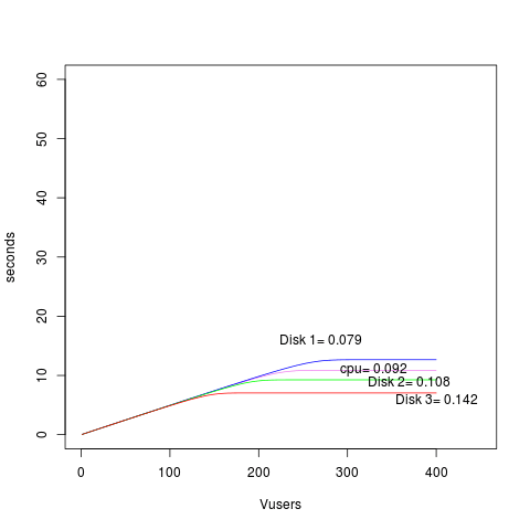
This simple script shows response time graphs of multiple devices in the same graph.

The second graph shows throughput curves. We just have to use GetThruput instead of GetResponse.

library(pdq)

# PDQ globals
load<-400
think<-20

cpu<-"cpunode"
disk1<-"disknode1"
disk2<-"disknode2"
disk3<-"disknode3"



cpudemand<-0.092
disk1demand<-0.079
disk2demand<-0.108
disk3demand<-0.142

workload<-"workload"

# R plot vectors
xc<-0
yc<-0

for (n in 1:load) {
	Init("")

	CreateClosed(workload, TERM, as.double(n), think)

	CreateNode(cpu, CEN, FCFS)
	SetDemand(cpu, workload, cpudemand)

	Solve(EXACT)

	xc[n]<-as.double(n)
	yc[n]<-GetResponse(TERM, workload)
}
plot(xc, yc, type="l", ylim=c(0,60), xlim=c(0,450), lwd=1, xlab="Vusers", ylab="seconds",col="violet")

text(370,13,paste("cpu-",as.numeric(cpudemand)))

# R plot vectors
xc1<-0
yc1<-0

for (n in 1:load) {
	Init("")

	CreateClosed(workload, TERM, as.double(n), think)

	CreateNode(disk1, CEN, FCFS)
	SetDemand(disk1, workload, disk1demand)

	Solve(EXACT)

	xc1[n]<-as.double(n)
	yc1[n]<-GetResponse(TERM, workload)
}
lines(xc1, yc1,lwd=1,col="blue")
text(400,10,paste("Disk 1-",as.numeric(disk1demand)))

# R plot vectors
xc2<-0
yc2<-0

for (n in 1:load) {
	Init("")

	CreateClosed(workload, TERM, as.double(n), think)

	CreateNode(disk2, CEN, FCFS)
	SetDemand(disk2, workload, disk2demand)

	Solve(EXACT)

	xc2[n]<-as.double(n)
	yc2[n]<-GetResponse(TERM, workload)
}
lines(xc2, yc2,lwd=1,col="green")
text(330,17,paste("Disk 2-",as.numeric(disk2demand)))

# R plot vectors
xc3<-0
yc3<-0

for (n in 1:load) {
	Init("")

	CreateClosed(workload, TERM, as.double(n), think)

	CreateNode(disk3, CEN, FCFS)
	SetDemand(disk3, workload, disk3demand)

	Solve(EXACT)

	xc3[n]<-as.double(n)
	yc3[n]<-GetResponse(TERM, workload)
}
lines(xc3, yc3,lwd=1,col="red")
text(240,20,paste("Disk 3-",as.numeric(disk3demand)))

Load vs Response

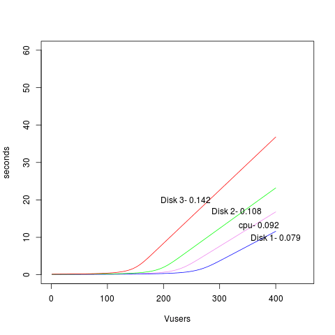
Load vs Throughput