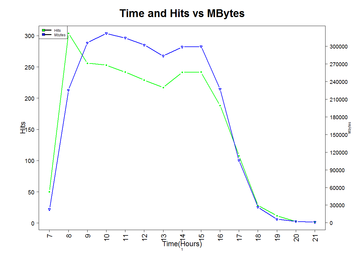
Graph of ‘Time and Hits vs MBytes’ using ‘R’

I am yet to crack the capacity planning method using statistical analysis but I am on my way to that exalted state of expertise.

Time and Hits vs MBytes

this.dir <- dirname(parent.frame(2)$ofile) 
setwd(this.dir)
 
 png(
"daily traffic-hits-bytes.png",
width =1200, height = 868)
par(mar=c(7, 9, 6, 8))
 
data = input <- readLines(textConnection("
07 22,864 27,574 49.79 MB 
08 225,337 252,366 303.75 MB 
09 306,007 318,463 256.01 MB 
10 322,103 331,298 252.89 MB 
11 314,393 322,646 241.72 MB 
12 302,438 309,236 228.91 MB 
13 283,773 290,291 217.17 MB 
14 299,020 306,326 241.34 MB 
15 299,792 307,692 241.76 MB 
16 227,502 232,658 188.31 MB 
17 106,205 108,890 107.65 MB 
18 26,589 27,667 28.13 MB 
19 5,952 6,143 11.72 MB 
20 2,212 2,213 2.49 MB 
21 937 944 1.33 MB"))
 
data <- read.table(text=data,sep=" ",header=FALSE,stringsAsFactors=FALSE,fill=TRUE)
data <- data.frame(data)
colnames(data) <- c("Hours", "Pages", "Hits", "Bandwidth")

plot(data$Hours,as.numeric(gsub(",","", data$Bandwidth)),col="green",pch=16,type="b", ylab="Hits", xlab="",las=2,lwd=2.5,xaxt="n", cex.lab=2,cex.axis=1.6)
axis(1,at = seq(min(data$Hours), max(data$Hours), by=1),las = 2,cex.axis=2)
title("Time and Hits vs MBytes",cex.main=3,xlab="Time(Hours)", cex.lab=2,1)
par(new=TRUE)
plot(data$Hours,as.numeric(gsub(",","",data$Pages)),yaxt="n",xlim=c(min(data$Hours),max(data$Hours)),col="blue",cex.axis=2.0,col.axis="blue",pch=6,type="b",xaxt="n",ylab="",xlab="",las=2,lwd=2.5, cex.lab=2)
mtext("Mbytes",side=4,line=5)
axis(4,at = seq(0, max(as.numeric(gsub(",","",data$Pages))), by=30000),las = 2,cex.axis=1.5)
legend("topleft", lty=c(1,1),lwd=c(3.5,3.5),c("Hits","Mbytes"), fill=c("green","blue"))
#box()
 
dev.off()