Processing unix ”pmap” output of a JVM

Analysis of the output of

pmap

using R seemed to take forever. The functional programming style did not help much. But the code with comments is below.

I plan to use this code as part of a ‘nmon’ data analyzer. Code will be in github soon.

@ Set the current directory so that the graphs are generated there
this.dir <- dirname(parent.frame(2)$ofile) 
setwd(this.dir) 



#Split unix 'pmap' output. This line is like black magic to me at this time.
d <- do.call(rbind, lapply(strsplit(readLines("D:\\Log analysis\\Process Maps\\pmap_5900"), "\\s+"), function(fields) c(fields[1:10], paste(fields[-(1:10)], collapse = " "))))

#Now I am assigning some columns names
colnames(d) <- c("Address","Kbytes","RSS","Dirty Mode","Mapping","Test6","Test7","Test8","Test9","Test10","Test11")

#This section isolates and graphs mainly 'anon' memory sizes


#Aggregate and sum by type of memory allocation to get cumulative size for each type
Type2 <- setNames(aggregate(as.numeric(d[,"Kbytes"]), by=list(d[,"Test6"]),FUN=sum,na.rm=TRUE),c("AllocationType","Size"))

#I don't want this line. The extra braces in the original file have been added to the columns separately
Type2 <-subset(Type2, Type2$AllocationType != "[")

#Create data frame and cleanse
x<-data.frame(d[,7],d[,6],d[,2])
y<-subset(x, x[1] != "NA")
z<-data.frame(y[1],y[3])

png(
  "anonymous1.jpg",
  width     = 6.25,
  height    = 3.50,
  units     = "in",
  res       = 600,
)
par(mar=c(7,4,1,0))

colnames(z) <- c("AllocationType","Size")

# Split into rows of 100 each. This is not generic.
Type1Split<-split(z, sample(rep(1:3, 100)))
size<-data.frame(Type1Split[[1]]$Size)
colnames(size)<-c("Size")

#Plot the first set
barplot(as.numeric(levels(size$Size)[size$Size]),ylim=c(0,2000), names.arg=(paste(Type1Split[[1]]$AllocationType,Type1Split[[1]]$Size,"kb",sep=" ")),space=6, width=2, xlim = c(0, 1500), ylab="Kbytes",cex.names=0.3,las=2)

dev.off()

png(
  "anonymous2.png",
  width     = 6.25,
  height    = 3.50,
  units     = "in",
  res       = 600,
)
par(mar=c(7,4,1,0))

size<-data.frame(Type1Split[[2]]$Size)
colnames(size)<-c("Size")

#Plot the second set

barplot(as.numeric(levels(size$Size)[size$Size]),ylim=c(0,2000), names.arg=(paste(Type1Split[[2]]$AllocationType,Type1Split[[2]]$Size,"kb",sep=" ")),space=6, width=2, xlim = c(0, 1500), ylab="Kbytes",cex.names=0.3,las=2)

dev.off()

png(
  "anonymous3.png",
  width     = 7.25,
  height    = 3.50,
  units     = "in",
  res       = 600,
)
par(mar=c(7,4,1,0))

size<-data.frame(Type1Split[[3]]$Size)
colnames(size)<-c("Size")

#Plot the third set

barplot(as.numeric(levels(size$Size)[size$Size]),ylim=c(0,2000), names.arg=(paste(Type1Split[[3]]$AllocationType,Type1Split[[3]]$Size,"kb",sep=" ")),space=5, width=2, xlim = c(0, 1600), ylab="Kbytes",cex.names=0.3,las=2)

dev.off()



#This section isolates and graphs memory size of files loaded by the JVM

set.seed(10)

Type2Split<-split(Type2, sample(rep(1:2, nrow(Type2)/2)))

png(
  "pmap-node2.png",
  width     = 6.20,
  height    = 3.50,
  units     = "in",
  res       = 600,
)
par(mar=c(7,4,1,0))

barplot(Type2Split[[1]]$Size, width=1,xlim=c(0,820),ylim = c(0, 15000), space=8, ylab="Kbytes",col=c("violet"),names.arg=(paste(Type2Split[[1]]$AllocationType,Type2Split[[1]]$Size,"kb",sep=" ")), cex.names=0.3,las=2)

dev.off()

png(
  "pmap-node3.png",
  width     = 6.20,
  height    = 3.10,
  units     = "in",
  res       = 800,
)
par(mar=c(8,4,1,0)+0.3)


barplot(Type2Split[[2]]$Size, width=1,xlim=c(0,880),ylim = c(0, 4000), space=8, ylab="Kbytes",col=c("violet"),names.arg=(paste(Type2Split[[2]]$AllocationType,Type2Split[[2]]$Size,"kb",sep=" ")), cex.names=0.3,las=2)

dev.off()

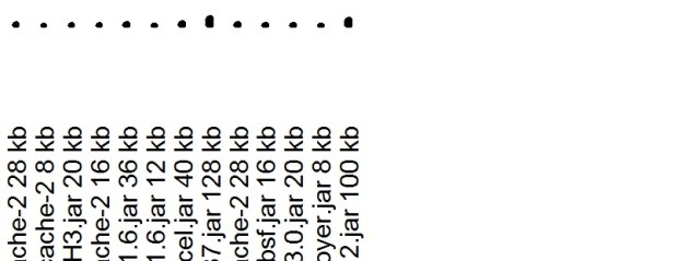
Graph of part of the JVM footprint showing files and memory sizes

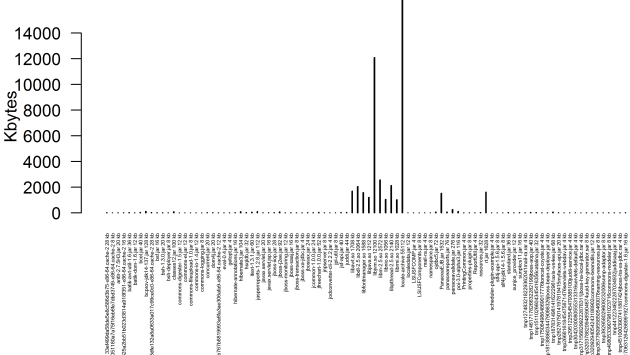
Blow up of the graph

Graph of the ‘anon’ and memory sizes which we thought was a problem

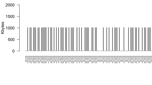
Blow up of the graph