Flow Matching and Diffusion Models
July 28, 2025 Leave a comment
I transcribe MIT 6.S184: Flow Matching and Diffusion Models – Lecture – Generative AI with SDEs. I try to do this using Tikz diagrams too.
tl:dr
- Ordinary Differential Equations have to be studied separately.
- Stochastic Differential Equations is a separate subject.
- I believe that I need to solve the exercises by coding to understand everything reasonably well.
Lecture 1
Conditional generation means sampling the conditional data distribution.

Generative models generate samples from data distribution.
Initial Distribution : 
Default is
Flow Model
Trajectory ![{ X : \overbrace{[0,1]}^\text{Time component} \rightarrow \mathbb{R}^D} , t \rightarrow X_t](https://s0.wp.com/latex.php?latex=%7B+X+%3A+%5Coverbrace%7B%5B0%2C1%5D%7D%5E%5Ctext%7BTime+component%7D+%5Crightarrow+%5Cmathbb%7BR%7D%5ED%7D+%2C+t+%5Crightarrow+X_t+&bg=f0f0f0&fg=555555&s=4&c=20201002)
Vector Field. ![{ u : \mathbb{R}^D x [0,1] \rightarrow \mathbb{R}^D}](https://s0.wp.com/latex.php?latex=%7B+u+%3A+%5Cmathbb%7BR%7D%5ED+x+%5B0%2C1%5D+%5Crightarrow+%5Cmathbb%7BR%7D%5ED%7D+&bg=f0f0f0&fg=555555&s=4&c=20201002)
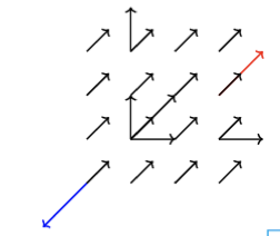
Flow
![{ \psi \bullet \mathbb{R}^D x [0,1] \rightarrow \mathbb{R}^D}](https://s0.wp.com/latex.php?latex=%7B+%5Cpsi+%5Cbullet+%5Cmathbb%7BR%7D%5ED+x+%5B0%2C1%5D+%5Crightarrow+%5Cmathbb%7BR%7D%5ED%7D+&bg=f0f0f0&fg=555555&s=4&c=20201002)


.The time derivative of 

Neural Network.
![{ {{\psi}_t}^{\theta} \mathbb{R}^D x [0,1] \rightarrow \mathbb{R}^D}](https://s0.wp.com/latex.php?latex=%7B+%7B%7B%5Cpsi%7D_t%7D%5E%7B%5Ctheta%7D+%5Cmathbb%7BR%7D%5ED+x+%5B0%2C1%5D+%5Crightarrow+%5Cmathbb%7BR%7D%5ED%7D+&bg=f0f0f0&fg=555555&s=4&c=20201002)
Random Initialization

Ordinary Differential Equation 
Goal Simulate to get


This means that Flow is a collection of Trajectories that conform to the ODE
Diffusion Model
Stochastic Process


![{ X : [0,1] \rightarrow \mathbb{R}^D , t \rightarrow X_t}](https://s0.wp.com/latex.php?latex=%7B+X+%3A+%5B0%2C1%5D+%5Crightarrow+%5Cmathbb%7BR%7D%5ED+%2C+t+%5Crightarrow+X_t%7D+&bg=f0f0f0&fg=555555&s=4&c=20201002)
Vector Field.
Stochastic Differential Equation

The following means that the change of 


Brownian Motion
Stochastic Process 

- It has Gaussian increments. What does it mean ?


These are two arbitrary time points and t is before s, 
3. Independent increments. This means that

So at this stage, in order to understand the following, I need a book or another course in ODE’s

This means the trajectory with ODE 


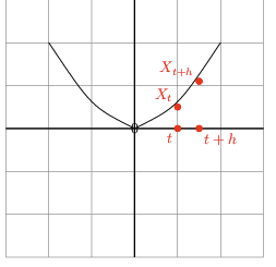
How are derivatives defined ?
This is the basic definition that I have to understand by learning Calculus.
Derivative of a trajectory 


And by applying linear algebra we get the ODE shown above( this section ).
Ordinary Differential Equation to Stochastic Differential Equation

![\Leftrightarrow X_{t+h} = X_t + h u_t (X_t) + \sigma_t \underbrace{(W_{t + h} - W_t)}_\text{Brownian Motion} + h R_t(h) \left( \displaystyle\lim_{h \to 0} \mathbb(E)[\sqrt {\lVert {R_t(h)} \rVert_2^2}] =0 \right)](https://s0.wp.com/latex.php?latex=%5CLeftrightarrow++++X_%7Bt%2Bh%7D++%3D+X_t+%2B+h+u_t+%28X_t%29+%2B+%5Csigma_t+%5Cunderbrace%7B%28W_%7Bt+%2B+h%7D+-+W_t%29%7D_%5Ctext%7BBrownian+Motion%7D+%2B+h+R_t%28h%29++%5Cleft%28+%5Cdisplaystyle%5Clim_%7Bh+%5Cto+0%7D+%5Cmathbb%28E%29%5B%5Csqrt+%7B%5ClVert+%7BR_t%28h%29%7D+%5CrVert_2%5E2%7D%5D+%3D0+%5Cright%29+&bg=f0f0f0&fg=555555&s=4&c=20201002)
This is the recap. We found a term that doesn’t depend on the derivatives that can be specified with an error term. 
Why do we need Brownian Motion ?
I didn’t really follow this. But the answer given was this. The Brownian Motion is equivalent to the Gaussian Distribution as far its universal value is concerned
Lecture 2
Reminder of what was covered in Lecture 1
![\fbox{\begin{minipage}[t][.5cm]{0,4\textwidth} {\textbf{Flow Model}} \end{minipage}} \qquad {P_{init}} {\textbf{(Gaussian)}} \qquad {d}X_t = \overbrace{{{u_t}^{\theta} (X_t) {dt} }^\text{{\textbf{ODE}}}}](https://s0.wp.com/latex.php?latex=%5Cfbox%7B%5Cbegin%7Bminipage%7D%5Bt%5D%5B.5cm%5D%7B0%2C4%5Ctextwidth%7D+%7B%5Ctextbf%7BFlow+Model%7D%7D+%5Cend%7Bminipage%7D%7D+%5Cqquad+%7BP_%7Binit%7D%7D+%7B%5Ctextbf%7B%28Gaussian%29%7D%7D+%5Cqquad+%7Bd%7DX_t+%3D+%5Coverbrace%7B%7B%7Bu_t%7D%5E%7B%5Ctheta%7D+%28X_t%29+%7Bdt%7D+%7D%5E%5Ctext%7B%7B%5Ctextbf%7BODE%7D%7D%7D%7D+&bg=f0f0f0&fg=555555&s=4&c=20201002)
![\fbox{\begin{minipage}[t][.8cm]{0,7\textwidth} \textbf{Diffusion Model} \end{minipage}} \qquad {P_{init}} {\textbf{(Gaussian)}} \qquad {d}X_t = \overbrace{ {u_t}^{\theta} (X_t){dt} + \underbrace{{\sigma}_t {d} W_t}_\text{{\textbf{Diffusion Co-efficient}}} }^\text{{\textbf{SDE}}}](https://s0.wp.com/latex.php?latex=%5Cfbox%7B%5Cbegin%7Bminipage%7D%5Bt%5D%5B.8cm%5D%7B0%2C7%5Ctextwidth%7D+%5Ctextbf%7BDiffusion+Model%7D+%5Cend%7Bminipage%7D%7D+%5Cqquad+%7BP_%7Binit%7D%7D+%7B%5Ctextbf%7B%28Gaussian%29%7D%7D+%5Cqquad+%7Bd%7DX_t+%3D+%5Coverbrace%7B+%7Bu_t%7D%5E%7B%5Ctheta%7D+%28X_t%29%7Bdt%7D+%2B+%5Cunderbrace%7B%7B%5Csigma%7D_t+%7Bd%7D+W_t%7D_%5Ctext%7B%7B%5Ctextbf%7BDiffusion+Co-efficient%7D%7D%7D+%7D%5E%5Ctext%7B%7B%5Ctextbf%7BSDE%7D%7D%7D+&bg=f0f0f0&fg=555555&s=4&c=20201002)
Deriving a Training Target
Typically, we train the model by minimizing a mean-squared error

In regression or classification, the training target is the label. Here we have no label. We have to derive a training target.
The professor states that you don’t have to understand all the derivations. I anticipate some mathematics I haven’t studied earlier.
We have to make sure we understand the formulas for these.
![\begin{minipage}[t][.6cm]{0.9\textwidth} {\textbf{Conditional \\ Probability Path}} \end{minipage} \qquad \begin{minipage}[t][.6cm]{0.9\textwidth} {\textbf{Conditional \\ Vector field}} \end{minipage} \qquad \begin{minipage}[t][.6cm]{0.9\textwidth} {\textbf{Conditional \\ Score Function}} \end{minipage}](https://s0.wp.com/latex.php?latex=%5Cbegin%7Bminipage%7D%5Bt%5D%5B.6cm%5D%7B0.9%5Ctextwidth%7D+%7B%5Ctextbf%7BConditional+%5C%5C+Probability+Path%7D%7D+%5Cend%7Bminipage%7D++%5Cqquad+%5Cbegin%7Bminipage%7D%5Bt%5D%5B.6cm%5D%7B0.9%5Ctextwidth%7D+%7B%5Ctextbf%7BConditional+%5C%5C+Vector+field%7D%7D+%5Cend%7Bminipage%7D+%5Cqquad+%5Cbegin%7Bminipage%7D%5Bt%5D%5B.6cm%5D%7B0.9%5Ctextwidth%7D+%7B%5Ctextbf%7BConditional+%5C%5C+Score+Function%7D%7D+%5Cend%7Bminipage%7D+&bg=f0f0f0&fg=555555&s=4&c=20201002)
![\begin{minipage}[t][.6cm]{0.9\textwidth} {\textbf{Marginal \\ Probability Path}} \end{minipage} \qquad \begin{minipage}[t][.6cm]{0.9\textwidth} {\textbf{Marginal \\ Vector field}} \end{minipage} \qquad \begin{minipage}[t][.6cm]{0.9\textwidth} {\textbf{Marginal \\ Score Function}} \end{minipage}](https://s0.wp.com/latex.php?latex=%5Cbegin%7Bminipage%7D%5Bt%5D%5B.6cm%5D%7B0.9%5Ctextwidth%7D+%7B%5Ctextbf%7BMarginal+%5C%5C+Probability+Path%7D%7D+%5Cend%7Bminipage%7D++%5Cqquad+%5Cbegin%7Bminipage%7D%5Bt%5D%5B.6cm%5D%7B0.9%5Ctextwidth%7D+%7B%5Ctextbf%7BMarginal+%5C%5C+Vector+field%7D%7D+%5Cend%7Bminipage%7D+%5Cqquad+%5Cbegin%7Bminipage%7D%5Bt%5D%5B.6cm%5D%7B0.9%5Ctextwidth%7D+%7B%5Ctextbf%7BMarginal+%5C%5C+Score+Function%7D%7D+%5Cend%7Bminipage%7D+&bg=f0f0f0&fg=555555&s=4&c=20201002)
The key terminology to remember are the following.
![\fbox{\begin{minipage}[t]{1,7\textwidth} \textbf{Conditional = Per Single data point \\ Marginal = Across distribution of data points } \end{minipage}}](https://s0.wp.com/latex.php?latex=%5Cfbox%7B%5Cbegin%7Bminipage%7D%5Bt%5D%7B1%2C7%5Ctextwidth%7D++%5Ctextbf%7BConditional+%3D+Per+Single+data+point+%5C%5C+Marginal+%3D+Across+distribution+of+data+points+%7D+%5Cend%7Bminipage%7D%7D++&bg=f0f0f0&fg=555555&s=4&c=20201002)
Conditional and Marginal Probability Path


This dirac distribution is not what I understand as of now. But it seems to return the same


Example : Gaussian Probability Path


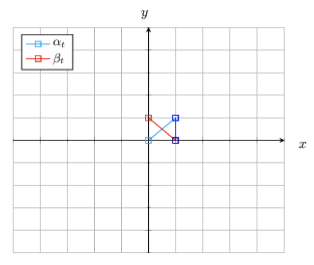
The diagram is small. But the idea is that when Time is 0, mean is 0 and variance is 1 which is 

The distributions with variance 1 is dirac,

Example : Marginal Probability Path 
Well. This is not clear at this stage. But we take one data point(sampling) from 


The density formula is not clear at this stage.
All of this seems to describe that we move from noise to our distribution of the data we are dealing with.

Conditional and Marginal Vector Field
Conditional Vector field 
We want to condition such that starting from initial point

then the distribution of t at every time point is given by this probablity path

We simulate the ODE like this.
Example : Conditional Gaussian Vector field


Marginalization trick
The marginal vector field is

Not very clear at this point but the following is the application of the bayes rule to look at the posterior distribution. What could have been the data point from the point set Z that gave rise to X ?


then the distribution of t at every time point is given by this marginal path

Conditional and marginal Score function
Conditional Score

Marginal Score

Derivation

Substituting the forumula show previously we get this after moving the gradient inside the integral.

Using the result


What is the score of the Conditional Gaussian Vector Field ?
This derivation is out of range for me at the moment but the instructor mentioned this.


Theorem : SDE extension trick


![{X_0 \sim {P_{init}}} , d{X_t} = \left[ {{u_t}^{target} (X_t)} + {\frac {{\alpha_t}^2}{2}} \nabla {\log {P_t( X_t )}} \right] dt + {\alpha_t} d{W_t} \Rightarrow {X_t \sim P_t}, {0 \leq t \leq 1}](https://s0.wp.com/latex.php?latex=%7BX_0+%5Csim+%7BP_%7Binit%7D%7D%7D+%2C+d%7BX_t%7D+%3D+%5Cleft%5B++%7B%7Bu_t%7D%5E%7Btarget%7D+%28X_t%29%7D+%2B+%7B%5Cfrac+%7B%7B%5Calpha_t%7D%5E2%7D%7B2%7D%7D+%5Cnabla+%7B%5Clog++%7BP_t%28+X_t+%29%7D%7D+%5Cright%5D+dt+%2B+%7B%5Calpha_t%7D+d%7BW_t%7D+%5CRightarrow+%7BX_t+%5Csim+P_t%7D%2C+%7B0+%5Cleq+t+%5Cleq+1%7D+&bg=f0f0f0&fg=555555&s=4&c=20201002)

